Pump and Probe: Time resolved ARPES
In this tutorial we show how to reconstruct the TR-ARPES spectral function in presence of excitons. See Refs.[1] [2]
ARPES from real-time propagation
The first part describes how to reconstruct the spectral function from after real-time propagation. If the real-time propagation has been done at the TD-HSEX level in a material with (strongly) bound excitons, and the pump pulse is tuned in resonance with an excitonic peak, the spectral function will show a fingerprint of the excitonic state, e.g. a replica of the valence band.
Store the history of the density matrix to disk
In order to reconstruct the ARPES response function, just run any real time propagation tutorial base on the `yambo_rt` executable (see for example this one: Real_time_Bethe-Salpeter_Equation_(density_matrix_only)) and add the following line to the input file
SaveGhistory
Please be aware that this will create a very large file containing the whole history of the density matrix. You can control how often the density matrix is written to disk with the second value in this input variable
% IOtime
 0.5 |5.0 |0.5 |  fs    # [RT] Time between to consecutive I/O (J,P,OCCs - GF - OUTPUT)
%
Usually the density matrix is used for restart only, and saving every 5 fs or so is reasonable. To reconstruct the TR-ARPES response function however, one needs to perform a Fourier transform, and it is usually need to write data more often to disk.
Run the real time simulation
yambo_rt -F inputs/td_run -J TD-RUN-NAME -C TD-RUN-NAME
Use the GKBA approach to reconstruct the spectral function
After the history is saved to disk, you can use `ypp_rt` to reconstruct the spectral function. Here an input file to be used to this end
TDplots                       # [R] Real-Time Post-Processing
RTGtwotimes                      # [R] Construct G<(t,tp)
RTtime                         # [R] Post-Processing kind: function of time
TimeStep= 0.01      fs      # Time step
% TimeRange
 25.00000 | 75.0000 | fs      # Time-window where processing is done
%
LoadGhistory                  # [NEGF] Build the NEQ density from the G_lesser
% EnRngeRt
 -2.00000 | 14.00000 | eV      # Energy range
%
ETStpsRt= 501                 # Total Energy steps
BuildGles
KeepCC        # This includes the contribiution from the c and c' terms of the density matrix in conduction

DampFactor= 50.0    meV
RhoDeph= 5.0    meV
INTERP_mode= "BOLTZ"              # Interpolation mode (NN=nearest point, BOLTZ=boltztrap aproach)
OutputAlat= 3.851738           # [a.u.] Lattice constant used for "alat" ouput format
cooIn= "rlu"                   # Points coordinates (in) cc/rlu/iku/alat
cooOut= "rlu"                  # Points coordinates (out) cc/rlu/iku/alat
INTERP_Shell_Fac= 20.00000     # The bigger it is a higher number of shells is used
#BANDS_path= "L G X"            # BANDS path points labels (G,M,K,L...)
BANDS_steps= 50                # Number of divisions
BANDS_built_in                 # Print the bands of the generating points of the circuit using the nearest internal point
%BANDS_kpts                    # K points of the bands circuit
   0.5000000 |  0.5000000 |  0.5000000 | #L(111)
   0.0000000 |  0.0000000 |  0.0000000 | #G
   0.0000000 |  0.5000000 |  0.5000000 | #X
%
You can also replace
BuildGles
with
BuildGret
Some extra options, which you can add to the input file, are available. For example
IncludeEQocc  # This includes the contribiution of the equilibrium occupations
KeepCV        # This includes the contribiution from the c and v  terms of the density matrix
KeepVC        # This includes the contribiution from the v and v' terms of the density matrix in valence
After your input file is ready just run
ypp_rt -F inputs/Gless_reconstruc -J "Gless,TD-RUN-NAME" -C TD-RUN-NAME
ARPES as BSE post processing
Warning: this is not yet available in the GPL release. You can download and use the following yambo fork if you are interested: https://gitlab.com/sangallidavide/lumen/-/tree/phys-excitons
In this second part we show instead how to simply reconstruct the spectral function from a post-porcessing of a BSE simulations at all transferred momenta in the IBZ. The BSE eigenvectors are needed. They can be obtained either via direct diagonalization or via iterative solvers like Slepc. The excitonic population is also needed as an input. The final spectral function will very similar to the real time approach if the population is assumed to be peaked at the bright excitonic state resonant with the pump pulse.
After solving BSE as discussed above, with `yambo_rt`
yambo_rt -F inputs/bse -J bse_allq -C bse_allq
just use the following input file (change it according to your needs) with `ypp_rt`
TDplots                          # [R] TD observables plot
TDplotmode                       # [R] TD plot control
RTARPES                          # [R] Transient ARPES
RTtime                           # [R] Post-Processing kind: function of time

% EnRngeRt
  8.00000 | 17.00000 | eV      # Energy range
%
ETStpsRt=  901                  # Total Energy steps
DampFactor= 0.10000       eV    # Damping parameter

Gauge= "length"                  # [RT] Gauge (length|velocity)
#FullExpansion

EXCTemp = 300.00 Kn
#TRabsNExc= 6
States= "1 - 100"                  # Index of the BS state(s)

INTERP_mode= "BOLTZ"              # Interpolation mode (NN=nearest point, BOLTZ=boltztrap aproach)
INTERP_Shell_Fac= 20.00000     # The bigger it is a higher number of shells is used
BANDS_path= "L,G,X"            # BANDS path points labels (G,M,K,L...)
BANDS_steps= 50                # Number of divisions
%BANDS_kpts                    # K points of the bands circuit
  0.5000000 |  0.5000000 |  0.5000000 | #L(111)
  0.0000000 |  0.0000000 |  0.0000000 | #G
  0.0000000 |  0.5000000 |  0.5000000 | #X
%
and finally run ypp_rt
ypp_rt -F inputs/arpes_from_bse -J "ARPES,bse_allq" -C ARPES
Below the output plotted with python using different excitonic distributions
- Reconstructed ARPES spectral function in LiF
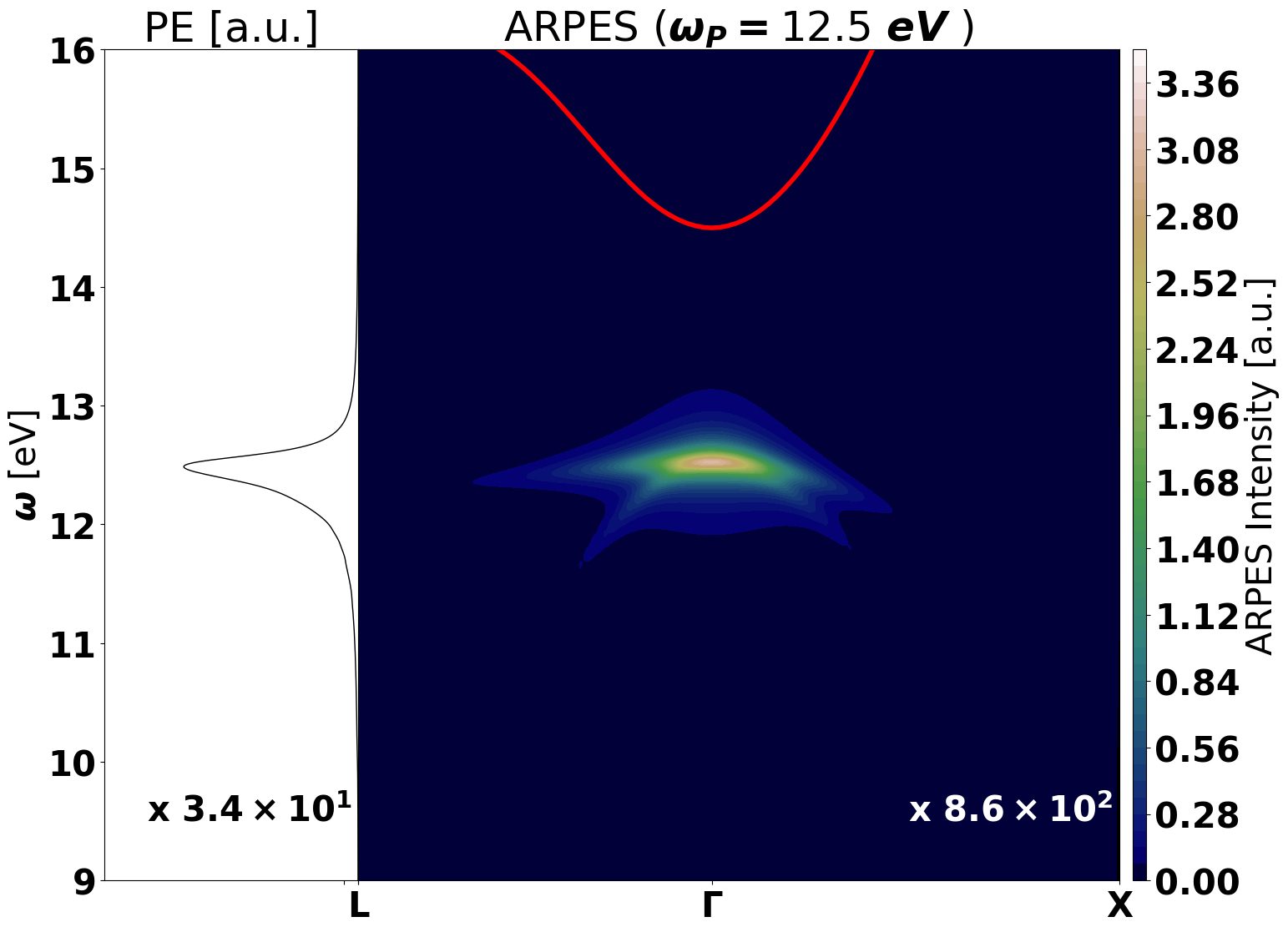
temperature T=0 K
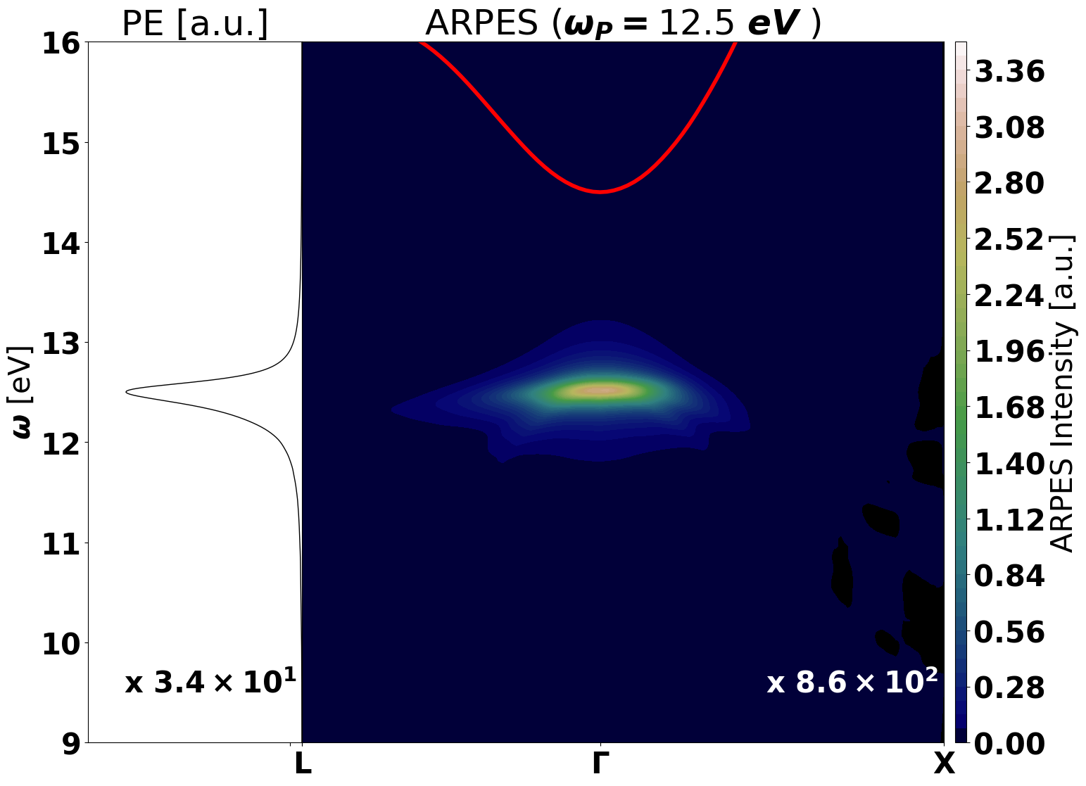
temperature T=300 K
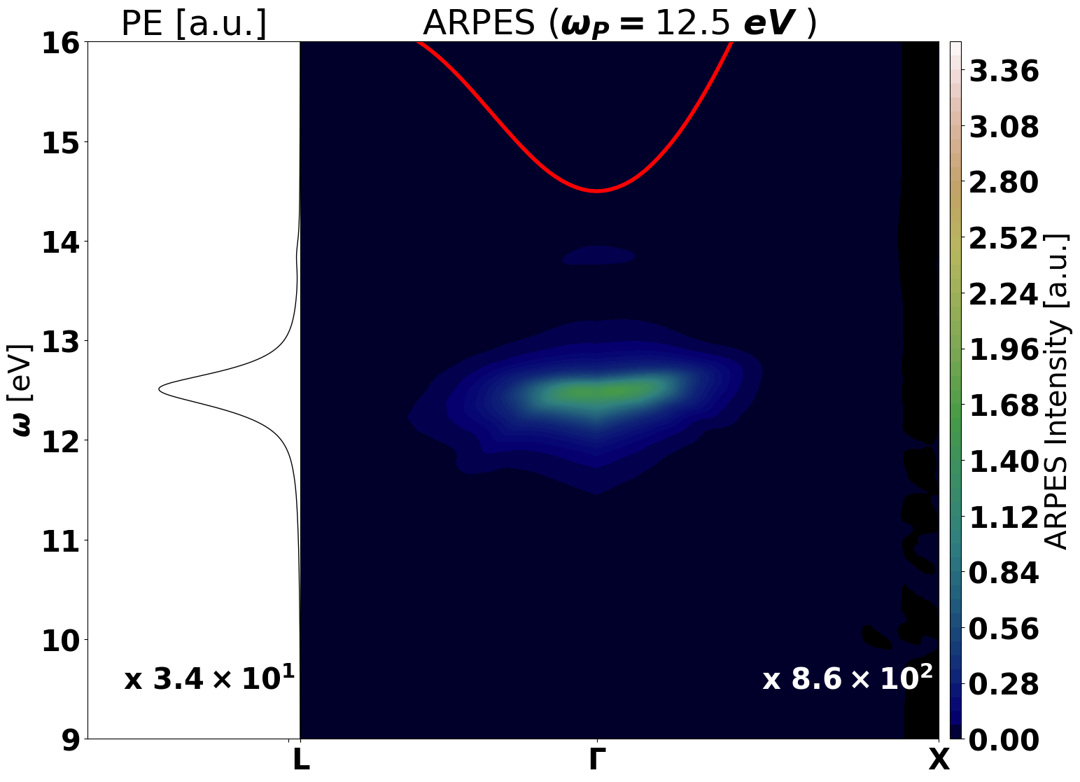
temperature T=3000 K


While at low temperature the signal is a replica of the valence band, at higher temperature the excitonic dispersion is obtained.
A similar feature was implemented in yambopy. See Ref.[3]
References
- ↑ E. Perfetto, D Sangalli, A Marini, G Stefanucci, Pump-driven normal-to-excitonic insulator transition: Josephson oscillations and signatures of BEC-BCS crossover in time-resolved ARPES, Physical Review Materials 3, 124601 (2019)
- ↑ D Sangalli, Excitons and carriers in transient absorption and time-resolved ARPES spectroscopy: An ab initio approach, Phys. Rev. Mat. 5, 083803 (2021)
- ↑ V. Gosetti, J. Cervantes-Villanueva, S. Mor, D. Sangalli, A. García-Cristóbal, et al., Unveiling exciton formation: exploring the early stages in time, energy and momentum domain preprint arXiv:2412.02507 (2025)