Bethe-Salpeter equation tutorial. Optical absorption (BN)
In this tutorial we will deal with different aspects of running a Bethe-Salpeter (BSE) calculation for optical absorption spectra using yambopy. We continue using hexagonal boron nitride to illustrate how to perform convergence tests, and how to compare and analyse the results.
Before you start this tutorial, make sure you have run the scf and nscf runs. If you have not, you can calculate the relax -r, scf -s and nscf -n using the gs_bn.py file:
$ python gs_bn.py -r -s -n
Once that is over, you can start the tutorial.
BSE convergence of optical spectra
In this section of the tutorial we will use the bse_conv_bn.py file. To evaluate the Bethe-Salpeter Kernel we need to first calculate the static dielectric screening, and then the screened Coulomb interaction matrix elements. This will be done with the file bse_conv_bn.py.
a. Static dielectric function
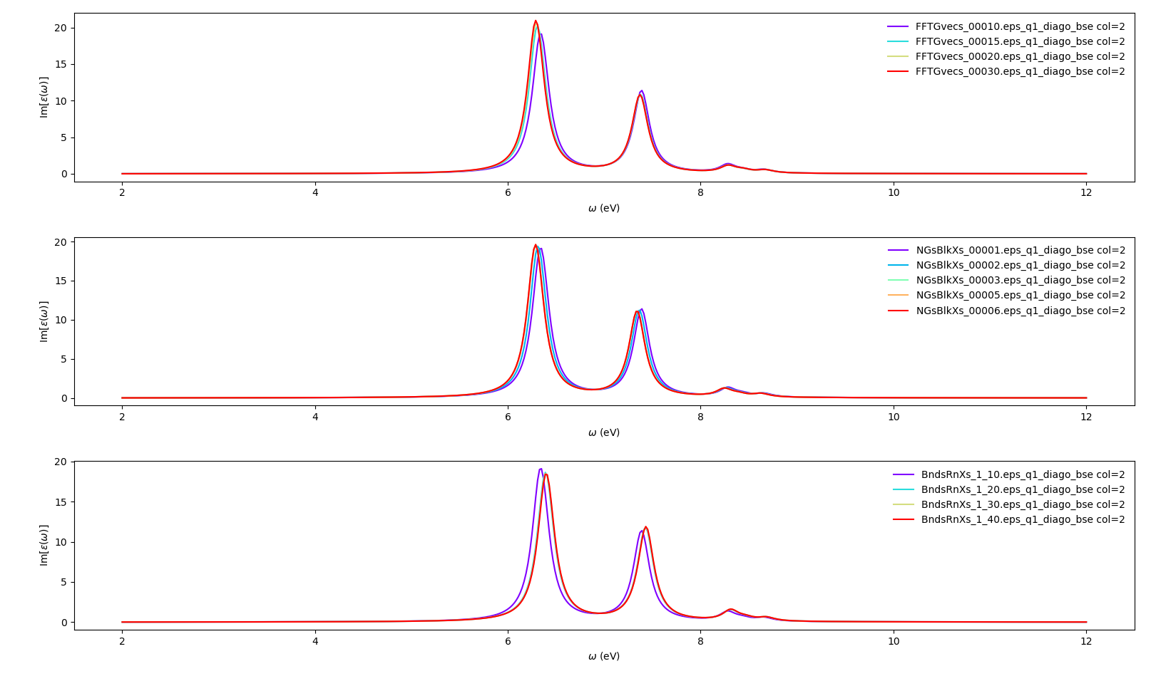
We begin by converging the static screening. In principle, all parameters can be converged independently one-by-one, and then the you can choose the best values for the final, fully converged result. To converge the static screening you will need:
FFTGvecs: number of planewaves to include. Usually we need fewer planewaves than the total used in the self-consistent cycle that generated the ground state in thescfrun. Reducing the total number of planewaves used diminishes the amount of memory per process that you are going to need.
BndsRnXs: number of bands to calculate the screening. Typically you need many bands (hundreds or even more) for the screening to converge.
NGsBlkXs: number of components for the local fields. Averages the value of the dielectric screening over a number of periodic copies of the unit cell. This parameter greatly increases the computational cost of the calculation and thus should be increased slowly.
We create a dictionary with different values for each variable. The python script (bse_conv_bn.py) will then create a reference input file with the first value in each parameter's list. It will then create input files with the other parameters changing independently according to the values specified on the list:
#list of variables to optimize the dielectric screening
conv = { 'FFTGvecs': [[10,10,15,20,30],'Ry'],
         'NGsBlkXs': [[1,1,2,3,5,6], 'Ry'],
         'BndsRnXs': [[1,10],[1,10],[1,20],[1,30],[1,40]] }
To run a calculation for each of the variables in the dictionary, we first define the run function
   def run(filename):
       """
       Function to be called by the optimize function
       """
       path = filename.split('.')[0]
       print(filename, path)
       shell = scheduler()
       shell.add_command('cd %s'%folder)
       shell.add_command('%s mpirun -np %d %s -F %s -J %s -C %s 2> %s.log'%(nohup,threads,yambo,filename,path,path,path))
       shell.add_command('touch %s/done'%path)
       if not os.path.isfile("%s/%s/done"%(folder,path)):
           shell.run()
which together with the optimize function in the class YamboIn,
y.optimize(conv,folder='bse_conv',run=run,ref_run=False)
will run and manage the calculations as defined in the dictionary. All calculation files and outputs will be in their respective directories inside the folder bse_conv.
To check which options are available in the script bse_conv_bn.py, run
$ python bse_conv_bn.py
which will give you the following list:
usage: bse_conv_bn.py [-h] [-r] [-a] [-p] [-e] [-b] [-u] [-t THREADS]

Test the yambopy script.

optional arguments:
  -h, --help            show this help message and exit
  -r, --run             run BSE convergence calculation
  -a, --analyse         analyse results data
  -p, --plot            plot the results
  -e, --epsilon         converge epsilon parameters
  -b, --bse             converge bse parameters
  -u, --nohup           run the commands with nohup
  -t THREADS, --threads THREADS
                        number of threads to use
So, in order to converge the screening, you will need to run
$ python bse_conv_bn.py -r -e
By default we have set up the total number of threads to be equal to 2. If you have access to more, you can change this using the -t option shown on the list, followed by the number of threads you want to use.
As you can see, the python script is running all the calculations changing the value of the input variables. You are free to open the bse_conv_bn.py file and modify it according to your own needs. Using the optimal parameters, you can run a calculation and save the dielectric screening databases ndb.em1s* to re-use them in the subsequent calculations. For that you can copy these files to the SAVE folder. yambo will only re-calculate any database if it does not find it or some parameter has changed.
Once the calculations are done you can plot resulting optical spectra by running
$ python bse_conv_bn.py -a
followed by
$ python bse_conv_bn.py -p -e
It will search the folder bse_conv for all calculations you performed previously and plot the results, using the class YamboAnalyser class.
Alternatively, you can obtain the same plots by running the the following script:
$ python plot-bse-conv.py
If you want to, you can now add new entries to the lists in the dictionary, specially the BndsRnXs, which usually requires a lot of bands to achieve convergence. Keep its number less than or equal to the number of bands in the nscf calculation, re-run the script and plot the results again. You can also test if some variables can converge with smaller values than the ones you used up to now.
b. Screened Coulomb interaction
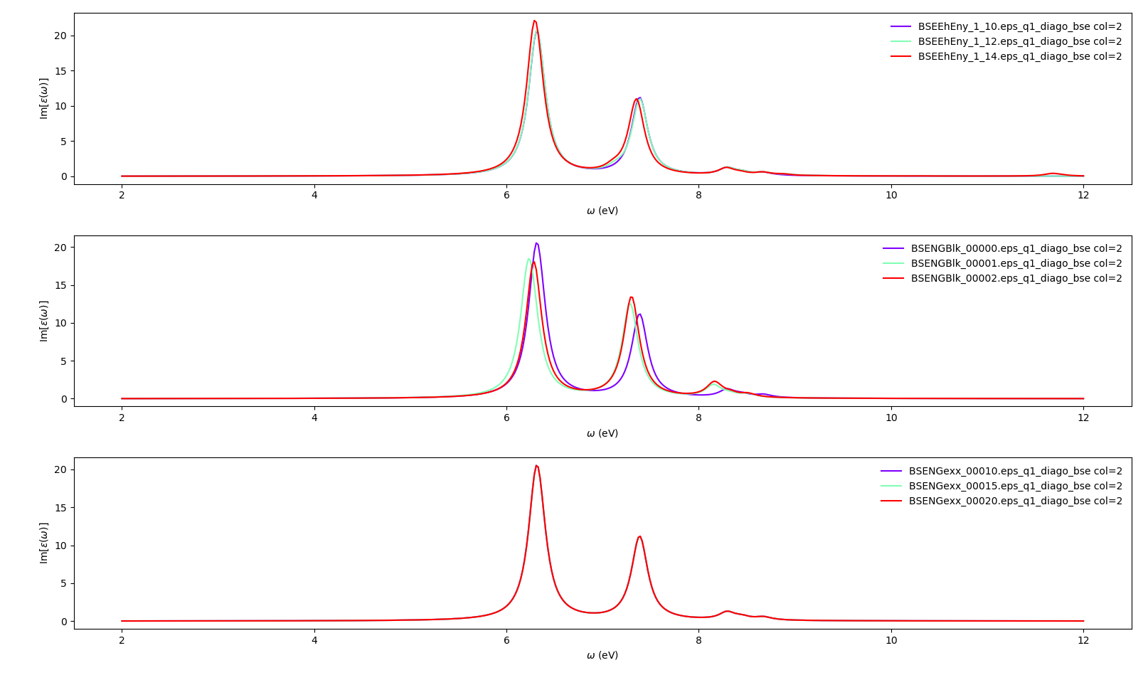
Up to this point we have been focused on the variables which control the static screening. We still need to deal with the variables which setup the Bethe-Salpeter auxiliary Hamiltonian matrix. Once this matrix is set up, yambo will use a diagonalisation algorithm to obtain the excitonic states and energies. The relevant variables for this process are:
BSEBands: number of bands to generate the transitions. Should be as small as possible as the size of the BSE auxiliary hamiltonian has (in the resonant approximation) dimensionsNk*Nv*Nc.Another way to converge the number of transitions is using
BSEEhEny. This variable selects the number of transitions based on the electron-hole energy difference (it's the one we are going to use).
BSENGBlkis the number of blocks for the dielectric screening average over the unit cells. This uses the static screening computed previously and controlled by the variableNGsBlkXs. So youBSENGBlkcannot be larger thanNGsBlkXs.
BSENGexxin the number of exchange components. Relatively cheap to calculate, but should be kept as small as possible to save memory.
KfnQP_Eis the scissor operator for the BSE. The first value is the rigid scissor, the second and third are the stretching for the conduction and valence respectively. The optical absorption spectrum is obtained in a range of energies given byBEnRangeand the number of frequencies in the interval isBEnSteps. Alternatively a quasiparticle energy database can be included from a previous GW calculation.
For the last variable you will be using a predefined scissor operator. If you want to know how to compute a scissor operator you can go and follow the GW tutorial here GW tutorial. Convergence and approximations (BN).
The dictionary of convergence in this case is:
#list of variables to optimize the BSE
        conv = { 'BSEEhEny': [[[1,10],[1,10],[1,12],[1,14]],'eV'],
                 'BSENGBlk': [[0,0,1,2], 'Ry'],
                 'BSENGexx': [[10,10,15,20],'Ry']}
All these variables do not change the dielectric screening, so optionally you can calculate it once (using the previous section to determine converged parameters) and put the database in the SAVE folder to make the calculations faster. Otherwise the dielectric screening will be computed for each run (in the case of this tutorial, this is still quite fast). This is a slightly advanced use of yambo, so it is better to leave till you are more familiar with the code and its flow.
To run the convergence calculations for the BSE Hamiltonian write:
$ python bse_conv_bn.py -r -b
Once the calculations are done you can plot the optical absorption spectra:
$ python bse_conv_bn.py -a
$ python bse_conv_bn.py -p -b
Alternatively, you can obtain the same plots by running the the following script: <source>$ python plot-bse-conv.py </source> Again, we invite you to change the values in the dictionary to check if the calculation would converge better using larger or smaller parameters.
Coulomb truncation convergence
a. Running for different layer separation distances
Here we will check how the dielectric screening changes with vacuum spacing between layers and including a coulomb truncation technique. For that we define a loop where we do a self-consistent ground state calculation, non self-consistent calculation, create the databases and run a yambo BSE calculation for different vacuum spacings.
To analyze the data we will plot the dielectric screening and check how the different values of the screening change the absorption spectra.
In the folder tutorials/bn/ you find the python script bse_cutoff_bn.py. This script takes some time to be executed, you can run both variants without the cutoff and with the cutoff -c simultaneously to save time. You can run this script with:
python bse_cutoff_bn.py -r -t4    # without coulomb cutoff
python bse_cutoff_bn.py -r -c -t4 # with coulomb cutoff
where -t specifies the number of MPI threads to use. The main loop changes the layer_separation variable using values from a list in the header of the file. In the script you can find how the functions scf, ncf and database are defined.
b. Plot the dielectric function
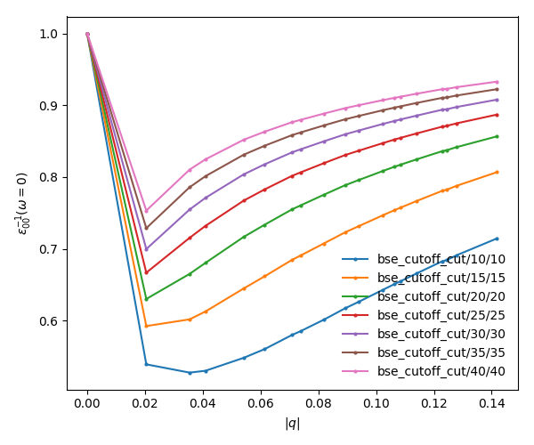
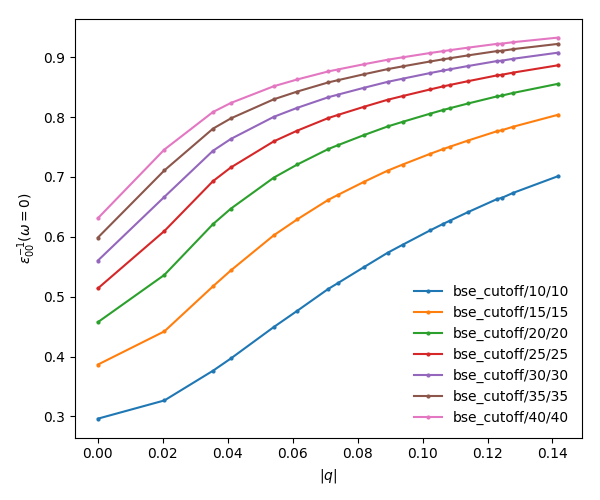
In a similar way as what was done before we can now plot the dielectric function for different layer separations:
yambopy plotem1s bse_cutoff/*/*     # without coulomb cutoff
yambopy plotem1s bse_cutoff_cut/*/* # with coulomb cutoff
In these figures it is clear that the long-range part of the coulomb interaction (q=0 in reciprocal space) is truncated, i. e. it is forced to go to zero.
c. Plot the absorption spectrum
You can also plot how the absorption spectra changes with the cutoff using:
python bse_cutoff_bn.py -p
python bse_cutoff_bn.py -p -c
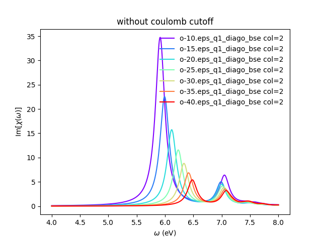
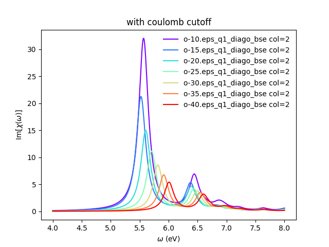
As you can see, the spectra is still changing with the vacuum spacing, you should increase the vacuum until convergence. For that you can add larger values to the layer_separations list and run the calculations and analysis again.
Excitonic wavefunctions in reciprocal space
In this example we show how to use yambopy to plot the excitonic wavefunction weights that result from a BSE calculation (specifically from the diagonalisation of the excitonic Hamiltonian). The script we will use this time is: bse_bn.py. Be aware the parameters specified for the calculation are not high enough to obtain a converged result.
To run the BSE calculation do:
python bse_bn.py -r
Alternatively, you can run
python bse_bn.py -r -c
to add the Coulomb cutoff.
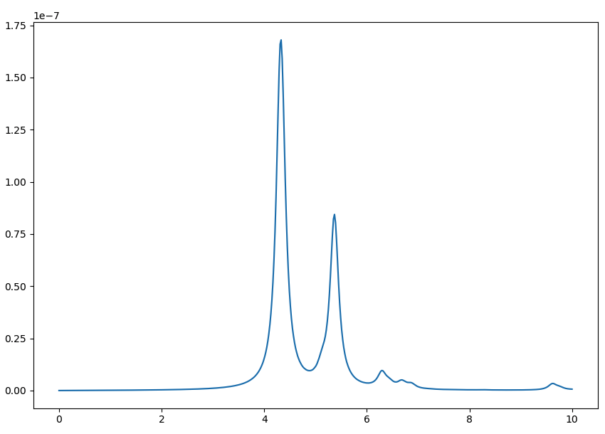
Then, the absorption spectrum is readily plotted by running the auxiliary script
python plot-bse.py
Afterwards you can run a basic analysis of the excitonic states and store the wavefunctions of the ones that are the most optically active, plotting them in reciprocal space. Plots in real space (not covered here) are also possible using yambopy (by calling ypp).
In order to proceed we will use the script plot-excitondb.py.
After running it as
python plot-excitondb.py
it will produce three plots.
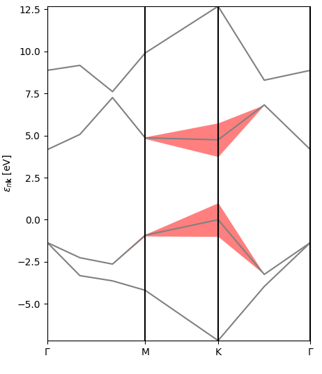
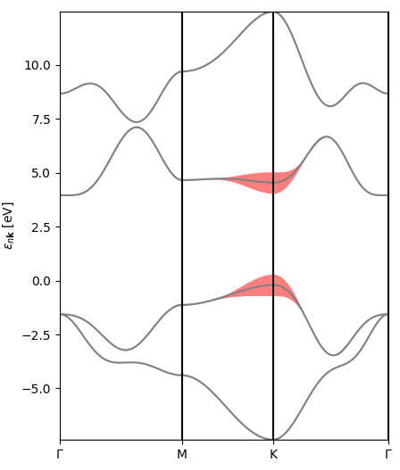
The first one is a representation of the excitonic weights (or rather their modulus) in reciprocal space, band- and kpoint-resolved, for the lowest-bound exciton. You can see that the electronic transitions contributing to this state originate mostly at symmetry point K (direct band gap) and along the KM line (the bands here have pi-type orbital character).
The second figure is an interpolated version of the first, with the bands and excitonic contributions appearing smoother.
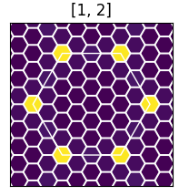
The final figure is a representation of the excitonic weights, summed over all bands, within the Brillouin zone. The brighter colors indicate where the most important electronic transitions for this excitonic state are located.
You can obtain plots for different excitonic states by changing the line
# List of states to be merged
states = [1,2]
in plot-excitondb.py.
You may also want to test the script with a more converged calculation: to this end you can increase the number of kpoints in the nscf calculation by going to gs_bn.py and changing the line
kpoints_nscf = [6,6,1]
to your liking (for example to 12x12x1).
Then, run again the following commands (nscf calculation, regeneration of yambo database, new BSE calculation).
python gs_bn.py -n
rm -r database
python bse_bn.py -r -t 4
As for the plotting, you may want to increase the value of lpratio in plot-excitondb.py to ensure that the interpolation works, as well as reduce the value of scale for a nicer plot in the hexagonal BN.
The lines to be changed are
exc_bands_inter = yexc.interpolate(save,path,states,lpratio=5,f=None,size=0.5,verbose=True)
and
yexc.plot_exciton_2D_ax(ax,states,mode='hexagon',limfactor=0.8,scale=160)
Then, you can run plot-excitondb.py again.
Again, be aware that these figures serve only to show the kind of representation that can be obtained with yambo, ypp and yambopy. Further convergence tests need to be performed to obtain accurate results, but that is left to the user.
