Bethe-Salpeter equation tutorial. Optical absorption (BN)

In this tutorial we will deal with different aspects of running a BSE calculation for optical absorption spectra using yambopy. Before you start this tutorial, make sure you did the scf and nscf runs. If you did not, you can calculate the scf -s and nscf -n using the gs_bn.py file:

<source lang="bash">python gs_bn.py -s -n</source> When that is done, you can start the tutorial.

Relevant parameters for the convergence

In this section of the tutorial we will use the bse_conv_bn.py file. To calculate the Bethe-Salpeter Kernel we need to first calculate the static dielectric screening and then the screened coulomb interaction matrix elements. The relevant convergence parameters for these two stages are:

a. Static dielectric function

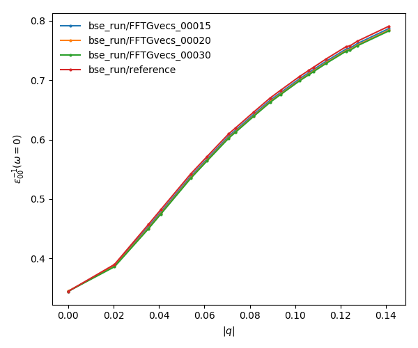
FFTGvecs: number of planewaves to include. Can be smaller than the number of planewaves in the self-consistency cycle. A typical good value is around 30 Ry (should always be checked!).

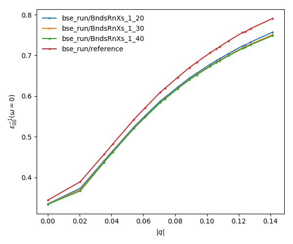
BndsRnXs: number of bands to calculate the screening. A very high number of bands is needed.

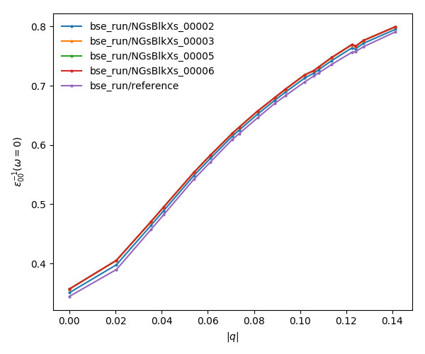
NGsBlkXs: number of components for the local fields. Averages the value of the dielectric screening over a number of periodic copies of the unit cell. This parameter increases greatly increases the cost of the calculation and hence should be increased slowly. A typical good value is 2 Ry.

To run the convergence we create a dictionary with different values for the variables. The python script (bse_conv_bn.py) will create a reference input file with the first value of each parameter. Then it will create input files with the other parameters changing according to the values specified in the list.

<source lang="python">#list of variables to optimize the dielectric screening conv = { 'FFTGvecs': [[10,15,20,30],'Ry'],

        'NGsBlkXs': [[1,2,3,5,6], 'Ry'],
        'BndsRnXs': [[1,10],[1,20],[1,30],[1,40]] }</source>

To run the convergence with the static dielectric function do:

<source lang="bash">python bse_conv_bn.py -r -e</source> As you can see, the python script is running all the calculations changing the value of the input variables. You are free to open the bse_conv_bn.py file and modify it accoridng to your own needs. Using the optimal parameters, you can run a calculation and save the dielectric screening databases ndb.em1s* to re-use them in the subsequent calculations. For that you can copy these files to the SAVE folder. yambo will only re-calculate any database if it does not find it or some parameter has changed.

Once the calculations are done you can plot the static dielectric function as a function of q points using the following commands:

<source lang="bash">yambopy plotem1s bse_conv/FFTGvecs* bse_conv/reference yambopy plotem1s bse_conv/BndsRnXs* bse_conv/reference yambopy plotem1s bse_conv/NGsBlkXs* bse_conv/reference</source>

You are at this point invited to add new entries to the list of BndsRnXs in the convergence dictionary (keep it bellow or equal to the number of bands in the nscf calculation) re-run the script and plot the results again.

b. Optical absorption spectra

Once you obtained a converged dielectric screening function you can calculate the Bethe-Salpeter auxiliary Hamiltonian and obtain the excitonic states and energies diagonalizing it or calculating the optical absorption spectra with a recursive technique like the Haydock method. Recall the relevant parameters for convergence:

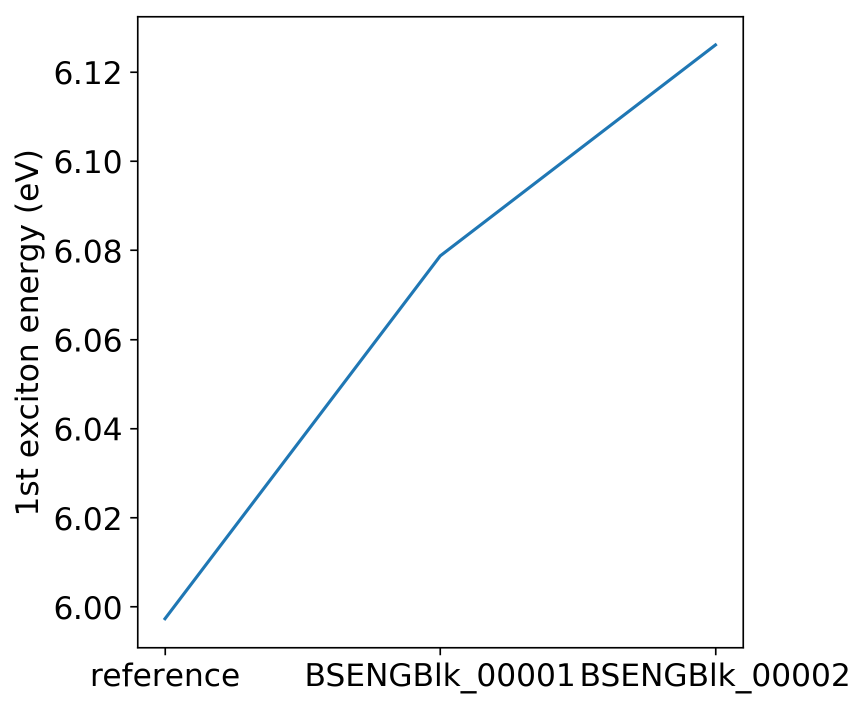
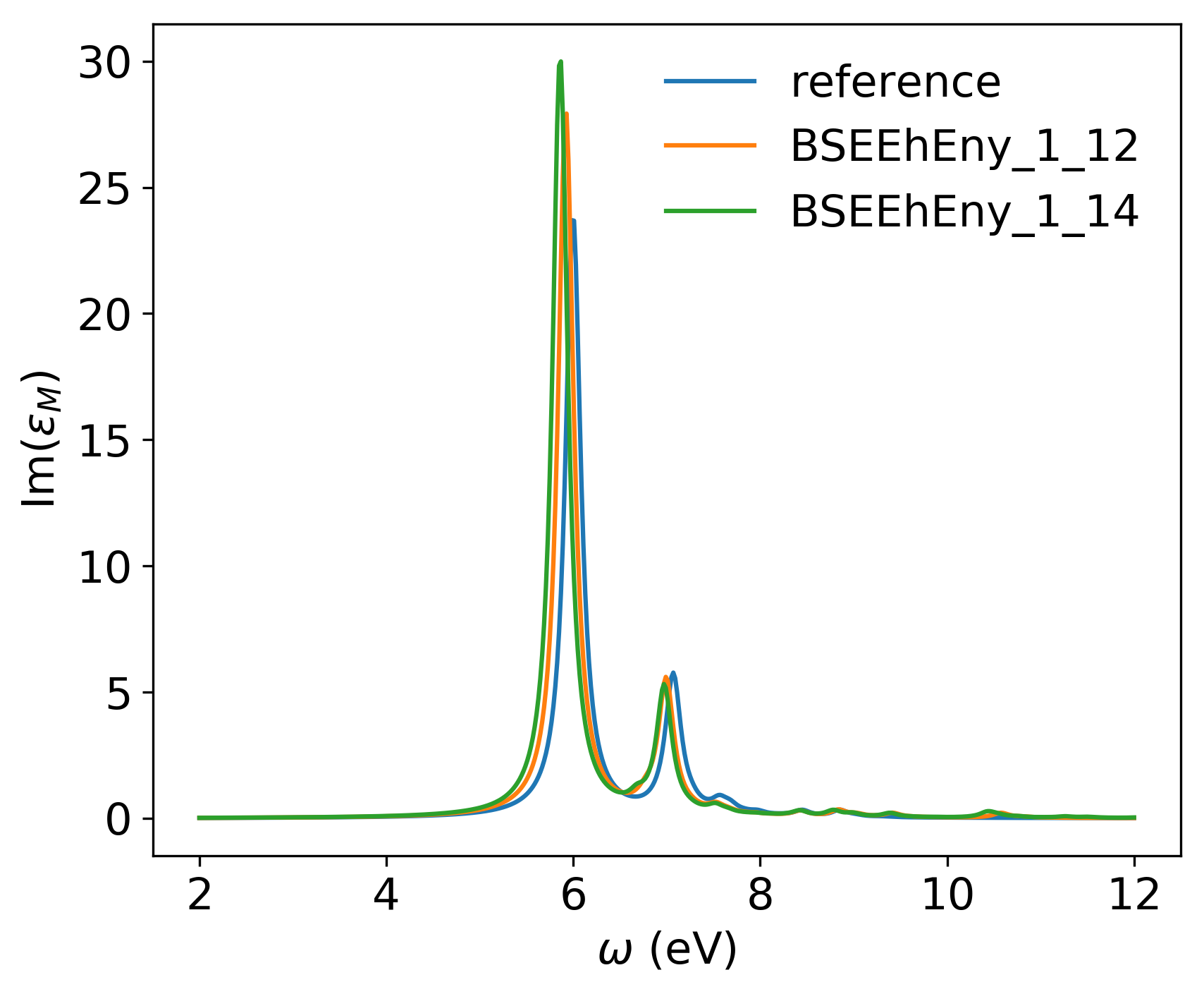
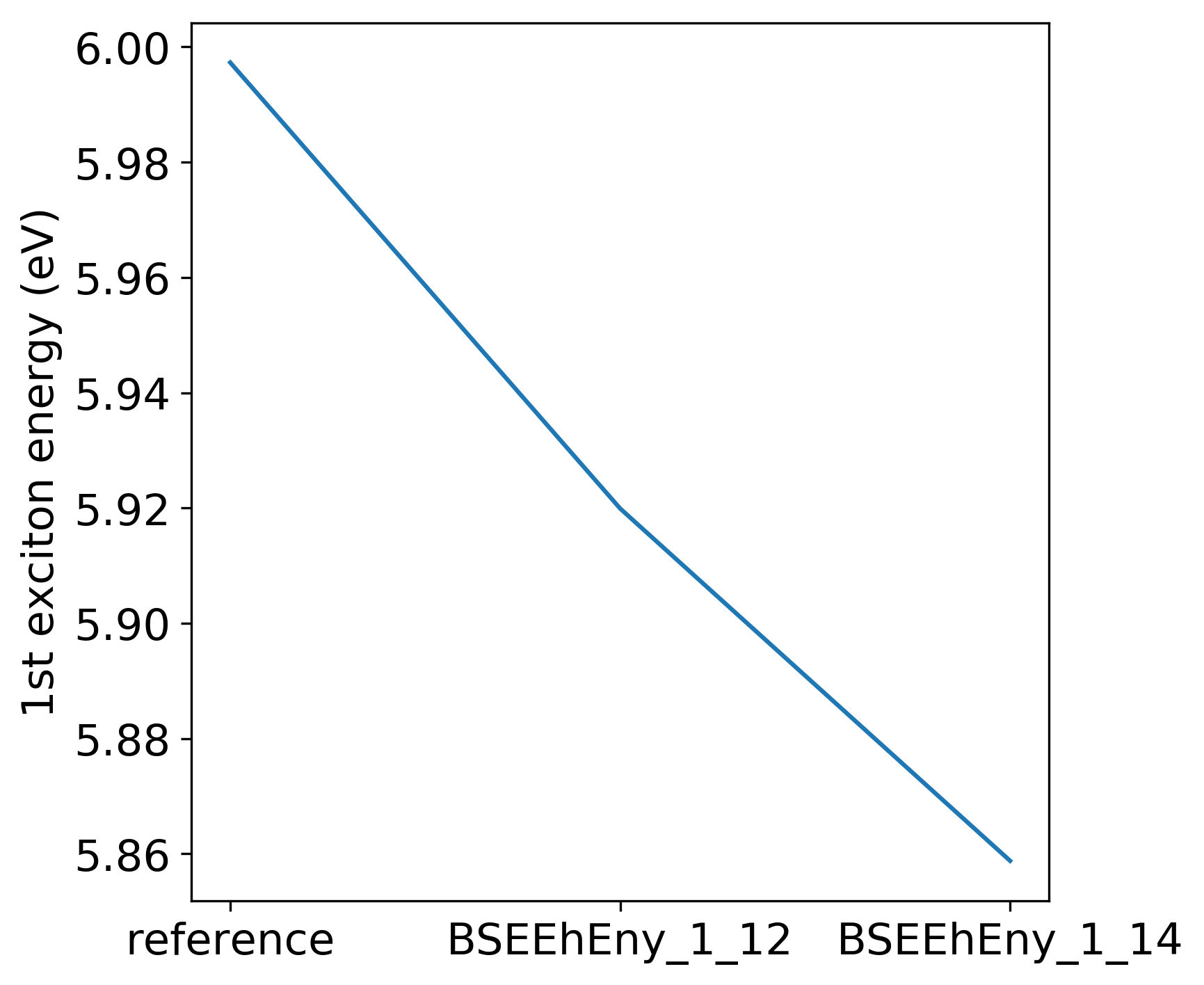
BSEBands: number of bands to generate the transitions. Should be as small as possible as the size of the BSE auxiliary hamiltonian has (in the resonant approximation) dimensions Nk*Nv*Nc. Another way to converge the number of transitions is using BSEEhEny. This variable selects the number of transitions based on the electron-hole energy difference.

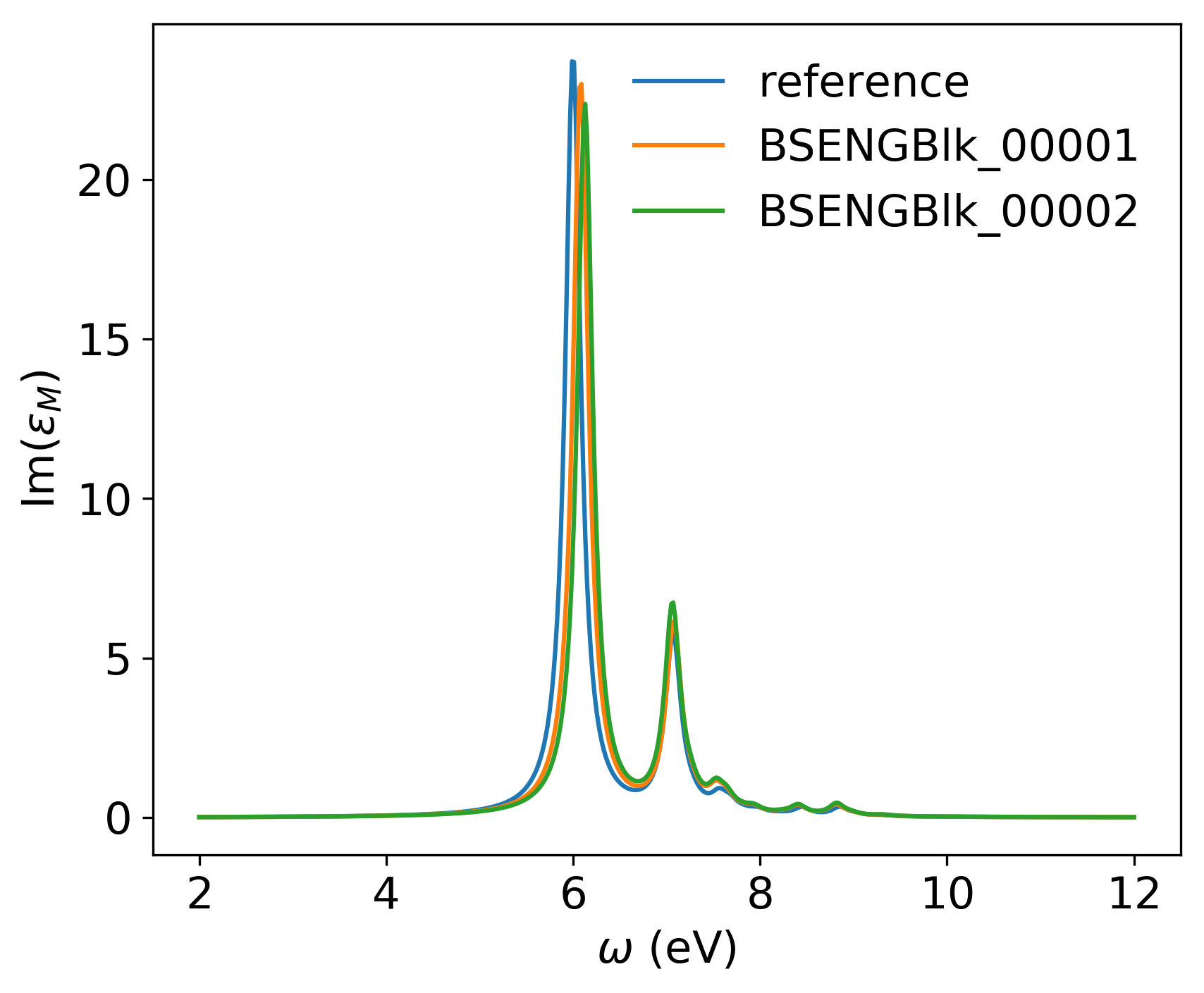
BSENGBlk is the number of blocks for the dielectric screening average over the unit cells. This has a similar meaning as NGsBlkXs.

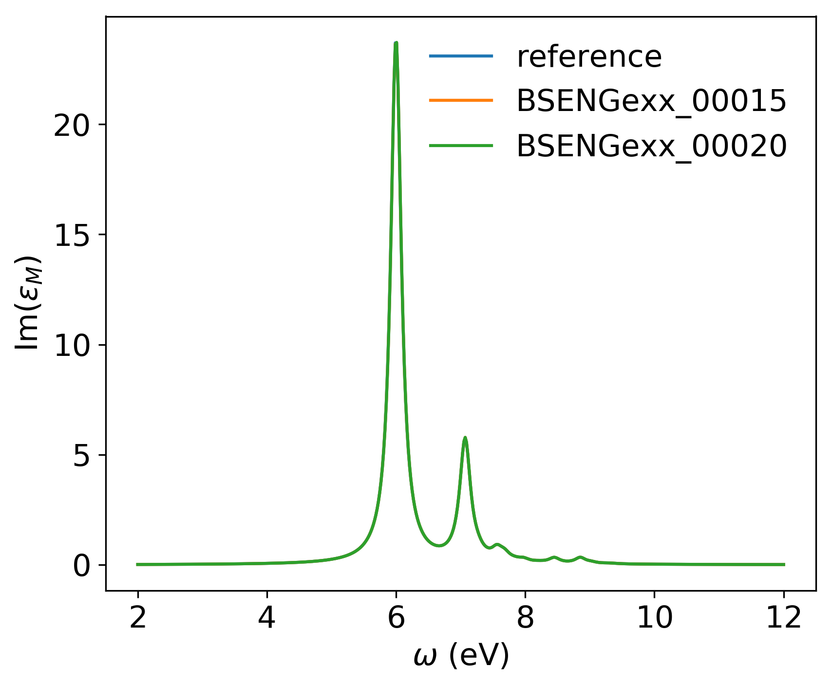
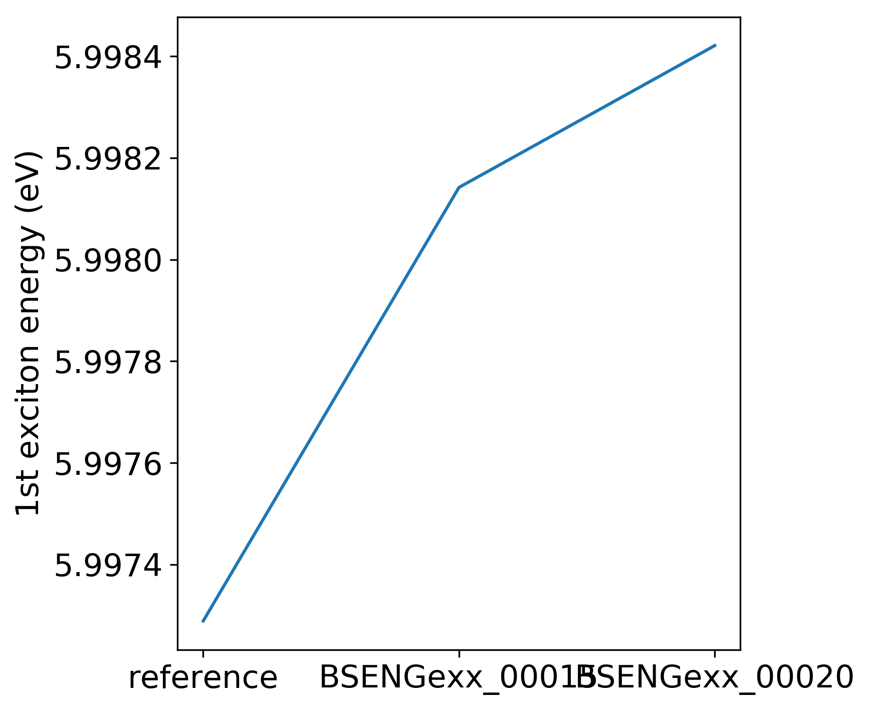
BSENGexx in the number of exchange components. Relatively cheap to calculate but should be as small as possible to save memory.

KfnQP_E is the scissor operator for the BSE. The first value is the rigid scissor, the second and third the stretching for the conduction and valence respectively. The optical absorption spectra is obtained in a range of energies given by BEnRange and the number of frequencies in the interval is BEnSteps.

The dictionary of convergence in this case is:

<source lang="python">#list of variables to optimize the BSE conv = { 'BSEEhEny': [[[1,10],[1,12],[1,14]],'eV'],

        'BSENGBlk': [[0,1,2], 'Ry'],
        'BSENGexx': [[10,15,20],'Ry']}</source>

All these variables do not change the dielectric screening, so you can calculate it once and put the database in the SAVE folder to make the calculations faster. To run these BSE part of the calculation do:

<source lang="bash">python bse_conv_bn.py -r -b</source> Once the calculations are done you can plot the optical absorption spectra:

<source lang="bash">yambopy analysebse bse_conv BSENGBlk yambopy analysebse bse_conv BSENGexx yambopy analysebse bse_conv BSEEhEny</source>

Coulomb truncation convergence

Here we will check how the dielectric screening changes with vacuum spacing between layers and including a coulomb truncation technique. For that we define a loop where we do a self-consistent ground state calculation, non self-consistent calculation, create the databases and run a yambo BSE calculation for different vacuum spacings.

To analyze the data we will plot the dielectric screening and check how the different values of the screening change the absorption spectra. In the folder tutorials/bn/ you find the python script bse_cutoff.py. This script takes some time to be executed, you can run both variants without the cutoff and with the cutoff -c simultaneously to save time. You can run this script with:

<source lang="bash">python bse_cutoff.py -r -t4 # without coulomb cutoff python bse_cutoff.py -r -c -t4 # with coulomb cutoff</source> where -t specifies the number of MPI threads to use. The main loop changes the layer_separation variable using values from a list in the header of the file. In the script you can find how the functions scf, ncf and database are defined.

3. Plot the dielectric function

In a similar way as what was done before we can now plot the dielectric function for different layer separations:

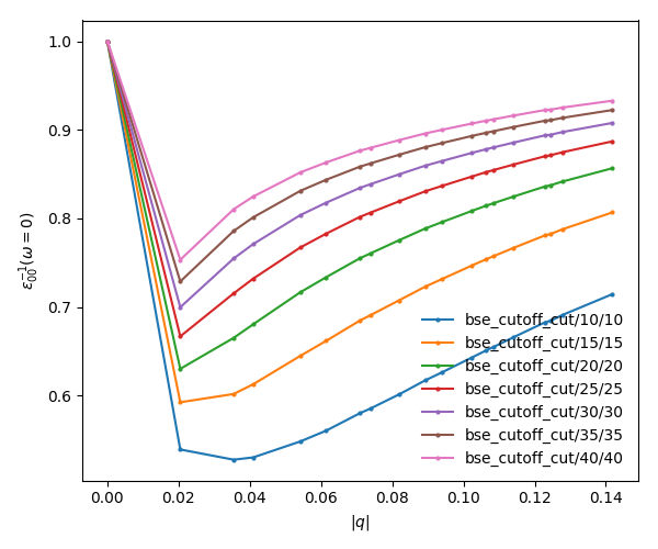
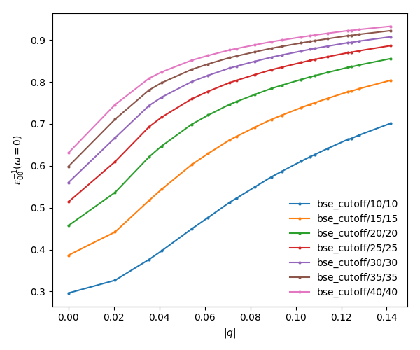
<source lang="bash">yambopy plotem1s bse_cutoff/*/* # without coulomb cutoff yambopy plotem1s bse_cutoff_cut/*/* # with coulomb cutoff</source>

In these figures it is clear that the long-range part of the coulomb interaction (q=0 in reciprocal space) is truncated, i. e. it is forced to go to zero.

2. Plot the absorption

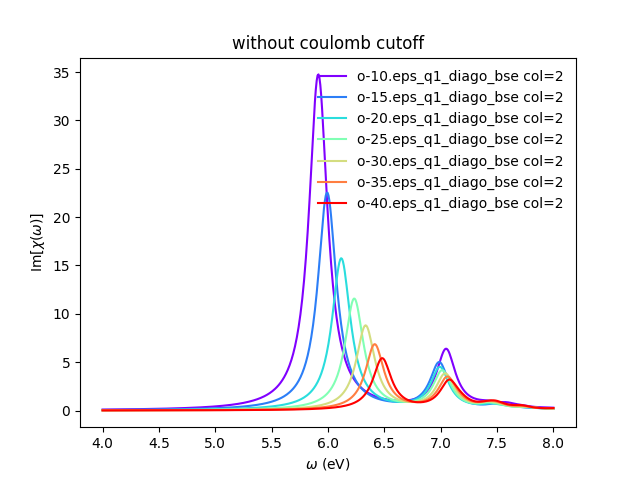
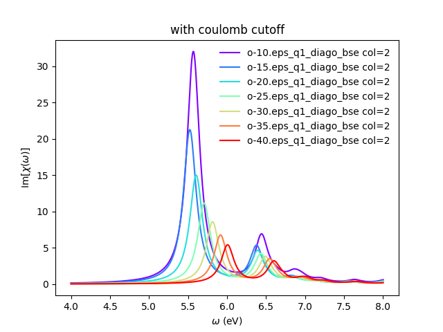
You can also plot how the absorption spectra changes with the cutoff using:

<source lang="bash">python bse_cutoff.py -p python bse_cutoff.py -p -c</source>

As you can see, the spectra is still changing with the vaccum spacing, you should increase the vacuum until convergence. For that you can add larger values to the layer_separations list and run the calculations and analysis again.

Excitonic wavefunctions

In this example we show how to use the yambopy to plot the excitonic wavefunctions that result from a BSE calculation. The script we will use this time is: bse_bn.py. Be aware the parameters specified for the calculation are not high enough to obtain a converged result. To run the BSE calculation do:

<source lang="bash">python bse_bn.py -r</source> Afterwards you can run a basic analysis of the excitonic states and store the wavefunctions of the ones that are more optically active and plot their wavefunctions in reciprocal space. Plots in real space are also possible using yambopy (by calling ypp). In the analysis code you have:

<source lang="python">#get the absorption spectra

1. 'yambo' : was the jobstring '-J' used when running yambo
2. 'bse'  : folder where the job was run

a = YamboBSEAbsorptionSpectra('yambo',path='bse')

1. Here we choose which excitons to read
2. min_intensity : choose the excitons that have at least this intensity
3. max_energy  : choose excitons with energy lower than this
4. Degen_Step  : take only excitons that have energies more different than Degen_Step

excitons = a.get_excitons(min_intensity=0.001,max_energy=7,Degen_Step=0.01)

1. read the wavefunctions
2. Cells=[13,13,1] #number of cell repetitions
3. Hole=[0,0,6+.5] #position of the hole in cartesian coordinates (Bohr units)
4. FFTGvecs=10 #number of FFT vecs to use, larger makes the
5. #image smoother, but takes more time to plot

a.get_wavefunctions(Degen_Step=0.01,repx=range(-1,2),repy=range(-1,2),repz=range(1),

                   Cells=[13,13,1],Hole=[0,0,6+.5], FFTGvecs=10,wf=True)

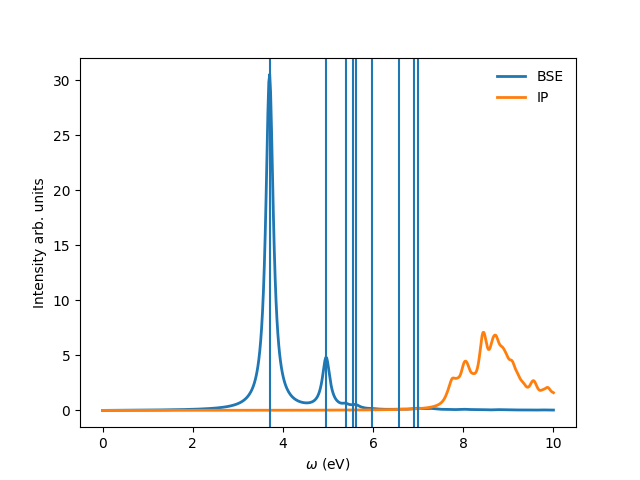
a.write_json()</source> The class YamboBSEAbsorptionSpectra() reads the absorption spectra obtained with explicit diagonalization of the BSE matrix. yambo if the job_string identifier used when running yambo, bse is the name of the folder where the job was run. The function get_excitons() runs ypp to obtain the exitonic states and their intensities. The function get_wavefunctions() also calls ypp and reads the reciprocal (and optionally real space) space wavefunctions and finally we store all the data in a json file.

This file can then be easily plotted with another python script. To run this part of the code you can do:

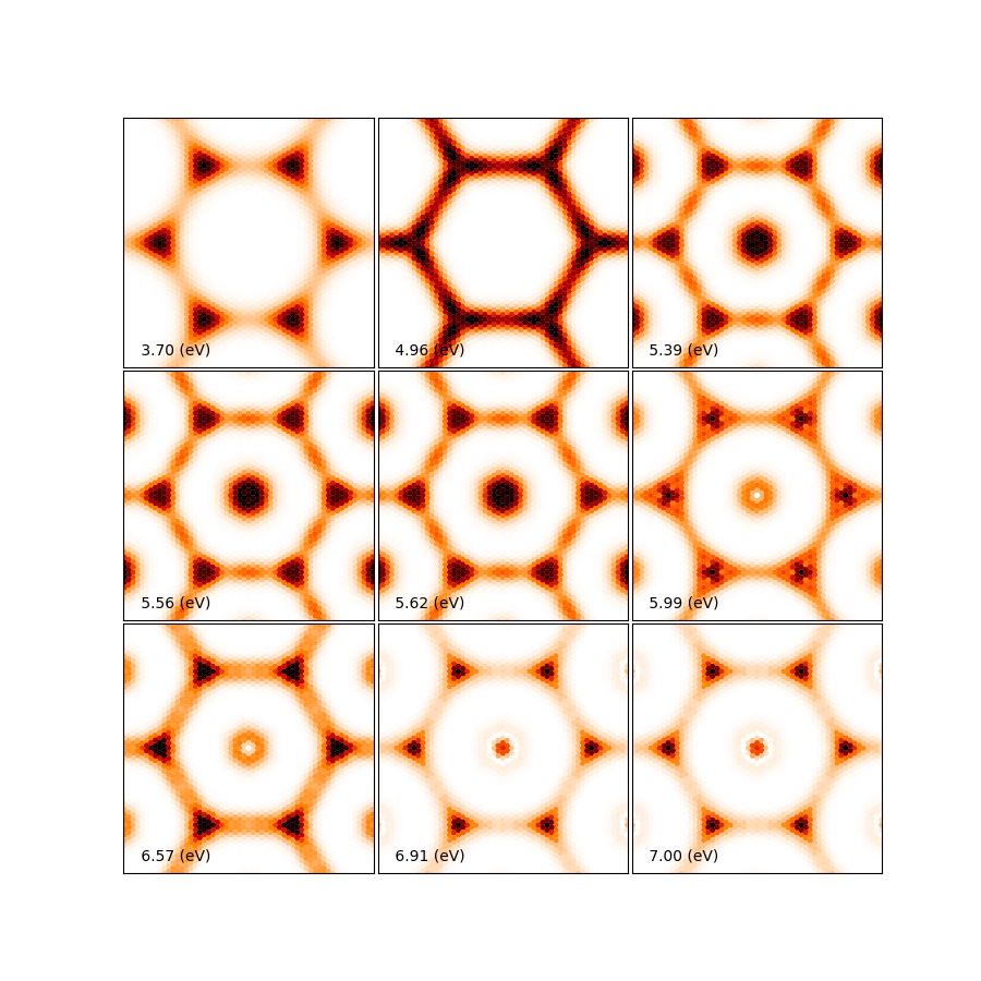
<source lang="bash">python bse_bn.py -a #this will generate absorptionspectra.json yambopy plotexcitons absorptionspectra.json #this will plot it</source> You can tune the parameters min_intensity and max_energy and obtain more or less excitons. Degen_Step is used to not consider excitons that are degenerate in energy. The reason is that when representing the excitonic wavefunction, degenerate states should be represented together. This value should in general be very small in order to not combine excitons that have energies close to each other but are not exactly degenerate. You should then obtain plots similar (these ones were generated on a 30x30 k-point grid) to the figures presented here:

Again, be aware that this figures serve only to show the kind of representation that can be obtained with yambo, ypp and yambopy. Further convergence tests need to be performed to obtain accurate results, but that is left to the user. You are invited to re-run the nscf loop with more k-points and represent the resulting wavefunctions.

You can now visualize these wavefunctions in real space using our online tool: http://henriquemiranda.github.io/excitonwebsite/

For that, go to the website, and in the Excitons section select absorptionspectra.json file using the Custom File. You should see on the right part the absorption spectra and on the left the representation of the wavefunction in real space. Alternatively you can vizualize the individually generated .xsf files using xcrysden.

Parallel static screening

In this tutorial we will show how you can split the calculation of the dielectric function in different jobs using yambopy. The dielectric function can then be used to calculate the excitonic states using the BSE.

The idea is that in certain clusters it is advantageous to split the jobs as much as possible. The dielectric function is calculated for different momentum transfer (q-points) over the brillouin zone. Each calculation is independent and can run at the same time. Using the yambo parallelization you can separate the dielectric function calculation among many cpus using the variable q in X_all_q_CPU and X_all_q_ROLEs. The issue is that you still need to make a big reservation and in some cases there is load imbalance (some nodes end up waiting for others). Splitting in smaller jobs can help your jobs to get ahead in the queue and avoid the load imbalance. If there are many free nodes you might end up running all the q-points at the same time.

The idea is quite simple: you create an individual input file for each q-point, submit each job separately, collect the results and do the final BSE step (this method should also apply for a GW calculation).

2. Parallel Dielectric function

To run the dielectric function in parallel do:

<source lang="bash">python bse_par_bn.py -r -t2</source> Here we tell yambo to calculate the dielectric function. We read the number of q-points the system has and generate one input file per q-point. Next we tell yambo to calculate the first q-point. yambo will calculate the dipoles and the dielectric function at the first q-point. Once the calculation is done we copy the dipoles to the SAVE directory. After that we run each q-point calculation as a separate job. Here the user can decide to submit one job per q-point on a cluster or use the python multiprocessing module to submit the jobs in parallel. In this example we use the second option.

<source lang="python">from yambopy import * import os import multiprocessing

yambo = "yambo"; folder = "bse_par"; nthreads = 2 #create two simultaneous jobs

1. create the yambo input file

y = YamboIn('yambo -r -b -o b -V all',folder=folder)

y['FFTGvecs'] = [30,'Ry'] y['NGsBlkXs'] = [1,'Ry'] y['BndsRnXs'] = [[1,30],] y.write('%s/yambo_run.in'%folder)

1. get the number of q-points

startk,endk = map(int,y['QpntsRXs'][0])

1. prepare the q-points input files

jobs = [] for nk in xrange(1,endk+1):

   y['QpntsRXs'] = [[nk,nk],]
   y.write('%s/yambo_q%d.in'%(folder,nk))
   if nk != 1:
       jobs.append('cd %s; %s -F yambo_q%d.in -J yambo_q%d -C yambo_q%d 2> log%d'%(folder,yambo,nk,nk,nk,nk))

1. calculate first q-point and dipoles

os.system('cd %s; %s -F yambo_q1.in -J yambo_q1 -C yambo_q1'%(folder,yambo))

1. copy dipoles to save

os.system('cp %s/yambo_q1/ndb.dip* %s/SAVE'%(folder,folder))

p = multiprocessing.Pool(nthreads) p.map(run_job, jobs)</source> 3. BSE

Once the dielectric function is calculated, it is time to collect the data in one folder and do the last step of the calculation: generate the BSE Hamiltonian, diagonalize it and calculate the absorption.

<source lang="python">#gather all the files if not os.path.isdir('%s/yambo'%folder):

   os.mkdir('%s/yambo'%folder)

os.system('cp %s/yambo_q1/ndb.em* %s/yambo'%(folder,folder)) os.system('cp %s/*/ndb.em*_fragment* %s/yambo'%(folder,folder))

y = YamboIn('yambo -r -b -o b -k sex -y d -V all',folder=folder) y['FFTGvecs'] = [30,'Ry'] y['NGsBlkXs'] = [1,'Ry'] y['BndsRnXs'] = [[1,30],] y['BSEBands'] = [[3,6],] y['BEnSteps'] = [500,] y['BEnRange'] = [[0.0,10.0],'eV'] y['KfnQP_E'] = [2.91355133,1.0,1.0] #some scissor shift y.arguments.append('WRbsWF') y.write('%s/yambo_run.in'%folder)

print('running yambo') os.system('cd %s; %s -F yambo_run.in -J yambo'%(folder,yambo))</source> 3. Collect and plot the results

You can then plot the data as before:

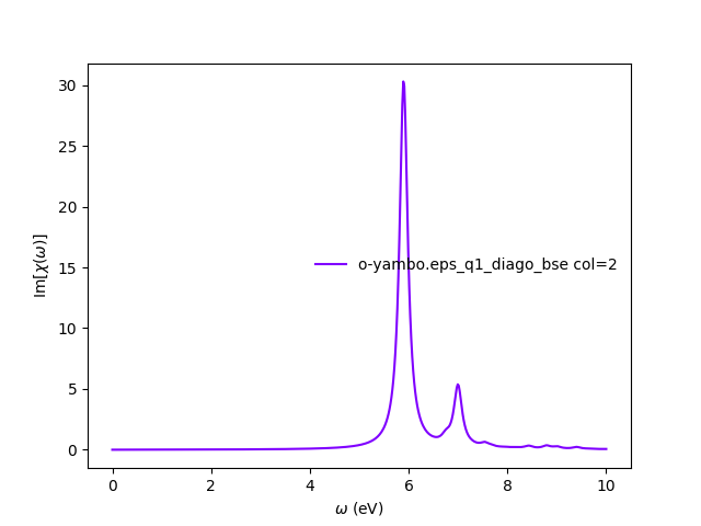
<source lang="bash">python bse_par_bn.py -p</source> This will execute the following code:

<source lang="python">#collect the data pack_files_in_folder('bse_par')

1. plot the results using yambo analyser

y = YamboAnalyser() print y y.plot_bse(['eps','diago'])</source> You should obtain a plot like this: