GW parallel strategies: Difference between revisions
| Line 15: | Line 15: | ||
To run a calculation on bellatrix you need to go via the queue system as explained in the Tutorials home. | To run a calculation on bellatrix you need to go via the queue system as explained in the Tutorials home. | ||
Under the YAMBO folder, together with the SAVE folder, you will see the | Under the YAMBO folder, together with the SAVE folder, you will see the run.sh script | ||
$ ls | $ ls | ||
| Line 68: | Line 68: | ||
and the submission script | and the submission script | ||
$ cat | $ cat run.sh | ||
#!/bin/bash | #!/bin/bash | ||
#SBATCH -N 1 | #SBATCH -N 1 | ||
| Line 75: | Line 75: | ||
#SBATCH -J test | #SBATCH -J test | ||
#SBATCH --reservation=cecam_course | #SBATCH --reservation=cecam_course | ||
#SBATCH --tasks-per-node=1 | #SBATCH --tasks-per-node=16 | ||
nodes=1 | |||
nthreads=1 | |||
ncpu=`echo $nodes $nthreads 16 | awk '{print $1*$3/$2}'` | |||
module purge | module purge | ||
module load intel/16.0.3 | module load intel/16.0.3 | ||
module load intelmpi/5.1.3 | module load intelmpi/5.1.3 | ||
bindir=/home/cecam.school/bin/ | |||
export OMP_NUM_THREADS= | |||
export OMP_NUM_THREADS=$nthreads | |||
label=MPI${ncpu}_OMP${nthreads} | |||
jdir=${ | jdir=run_${label} | ||
cdir=${ | cdir=run_${label}.out | ||
filein0=yambo_gw.in | filein0=yambo_gw.in | ||
filein=yambo_gw_${label}.in | filein=yambo_gw_${label}.in | ||
cp -f $filein0 $filein | cp -f $filein0 $filein | ||
cat >> $filein << EOF | cat >> $filein << EOF | ||
X_all_q_CPU= "1 1 $ncpu 1" | X_all_q_CPU= "1 1 $ncpu 1" # [PARALLEL] CPUs for each role | ||
X_all_q_ROLEs= "q k c v" | X_all_q_ROLEs= "q k c v" # [PARALLEL] CPUs roles (q,k,c,v) | ||
X_all_q_nCPU_LinAlg_INV= $ncpu # [PARALLEL] CPUs for Linear Algebra | |||
X_Threads= 0 # [OPENMP/X] Number of threads for response functions | X_Threads= 0 # [OPENMP/X] Number of threads for response functions | ||
DIP_Threads= 0 # [OPENMP/X] Number of threads for dipoles | DIP_Threads= 0 # [OPENMP/X] Number of threads for dipoles | ||
SE_CPU= " 1 1 $ncpu" | SE_CPU= " 1 1 $ncpu" # [PARALLEL] CPUs for each role | ||
SE_ROLEs= "q qp b" | SE_ROLEs= "q qp b" # [PARALLEL] CPUs roles (q,qp,b) | ||
SE_Threads= 0 | SE_Threads= 0 | ||
EOF | EOF | ||
echo "Running on $ncpu MPI, $nthreads OpenMP threads" | echo "Running on $ncpu MPI, $nthreads OpenMP threads" | ||
srun -n $ncpu -c $nthreads $bindir/yambo -F $filein -J $jdir -C $cdir | srun -n $ncpu -c $nthreads $bindir/yambo -F $filein -J $jdir -C $cdir | ||
| Line 109: | Line 114: | ||
As soon as you are ready submit the job. | As soon as you are ready submit the job. | ||
$ sbatch | $ sbatch run.sh | ||
Yambo calculates the GW-qp corrections running on 1 MPI process with a single thread. | Yambo calculates the GW-qp corrections running on 1 MPI process with a single thread. | ||
Revision as of 21:01, 25 April 2017
In this tutorial we will see how to setup the variables governing the parallel execution of yambo in order to perform efficient calculations in terms of both cpu time and memory to solution. As a test case we will consider the hBN 2D material. Because of its reduced dimensionality, GW calculations turns out to be very delicate. Beside the usual convergence studies with respect to k-points and sums-over-bands, in low dimensional systems a sensible amount of vacuum is required in order to treat the system as isolated, translating into a large number of plane-waves. As for other tutorials, it is important to stress that this tutorial it is meant to illustrate the functionality of the key variables and to run in reasonable time, so it has not the purpose to reach the desired accuracy to reproduce experimental results. Moreover please also note that scaling performance illustrated below may be significantly dependent on the underlying parallel architecture. Nevertheless, general considerations are tentatively drawn in discussing the results.
Getting familiar with yambo in parallel
If you are not inside bellatrix, please follow the instructions in the tutorial home. If you are inside bellatrix and in the proper folder
[cecam.school01@bellatrix yambo_YOUR_NAME]$ pwd
/scratch/cecam.schoolXY/yambo_YOUR_NAME
you can proceed. First you need to obtain the appropriate tarball
$ cp /scratch/cecam.school/hBN-2D-para.tar.gz  ./  (Notice that this time there is not XY!)
$ tar -zxvf hBN-2D-para.tar.gz
$ ls
YAMBO_TUTORIALS
$ cd YAMBO_TUTORIALS/hBN-2D/YAMBO
To run a calculation on bellatrix you need to go via the queue system as explained in the Tutorials home. Under the YAMBO folder, together with the SAVE folder, you will see the run.sh script
$ ls
parse_yambo.py  run.sh  SAVE
First run the initialization as usual. Then you need to generate the input file for a GW run.
$ yambo -g n - p
The new input file should look like the folllowing. Please remove the lines you see below with a stroke and set the parameters to the same values as below
$ cat yambo_gw.in # # # Y88b / e e e 888~~\ ,88~-_ # Y88b / d8b d8b d8b 888 | d888 \ # Y88b/ /Y88b d888bdY88b 888 _/ 88888 | # Y8Y / Y88b / Y88Y Y888b 888 \ 88888 | # Y /____Y88b / YY Y888b 888 | Y888 / # / / Y88b / Y888b 888__/ `88_-~ # # # GPL Version 4.1.2 Revision 120 # MPI+OpenMP Build # http://www.yambo-code.org # ppa # [R Xp] Plasmon Pole Approximation gw0 # [R GW] GoWo Quasiparticle energy levels HF_and_locXC # [R XX] Hartree-Fock Self-energy and Vxc em1d # [R Xd] Dynamical Inverse Dielectric MatrixX_Threads= 32 # [OPENMP/X] Number of threads for response functionsDIP_Threads= 32 # [OPENMP/X] Number of threads for dipolesSE_Threads= 32 # [OPENMP/GW] Number of threads for self-energyEXXRLvcs= 21817 RL # [XX] Exchange RL components Chimod= "" # [X] IP/Hartree/ALDA/LRC/BSfxc % BndsRnXp 1 | 200 | # [Xp] Polarization function bands % NGsBlkXp= 4 Ry # [Xp] Response block size % LongDrXp 1.000000 | 0.000000 | 0.000000 | # [Xp] [cc] Electric Field % PPAPntXp= 27.21138 eV # [Xp] PPA imaginary energy % GbndRnge 1 | 200 | # [GW] G[W] bands range % GDamping= 0.10000 eV # [GW] G[W] damping dScStep= 0.10000 eV # [GW] Energy step to evaluate Z factors DysSolver= "n" # [GW] Dyson Equation solver ("n","s","g") %QPkrange # [GW] QP generalized Kpoint/Band indices 1| 1| 3| 6| %
and the submission script
$ cat run.sh

#!/bin/bash
#SBATCH -N 1
#SBATCH -t 06:00:00
#SBATCH -J test
#SBATCH --reservation=cecam_course
#SBATCH --tasks-per-node=16

nodes=1
nthreads=1
ncpu=`echo $nodes $nthreads 16 | awk '{print $1*$3/$2}'`

module purge
module load intel/16.0.3
module load intelmpi/5.1.3
bindir=/home/cecam.school/bin/

export OMP_NUM_THREADS=$nthreads

label=MPI${ncpu}_OMP${nthreads}
jdir=run_${label}
cdir=run_${label}.out

filein0=yambo_gw.in
filein=yambo_gw_${label}.in

cp -f $filein0 $filein
cat >> $filein << EOF
X_all_q_CPU= "1 1 $ncpu 1"  # [PARALLEL] CPUs for each role
X_all_q_ROLEs= "q k c v"    # [PARALLEL] CPUs roles (q,k,c,v)
X_all_q_nCPU_LinAlg_INV= $ncpu   # [PARALLEL] CPUs for Linear Algebra
X_Threads=  0               # [OPENMP/X] Number of threads for response functions
DIP_Threads=  0             # [OPENMP/X] Number of threads for dipoles
SE_CPU= " 1 1 $ncpu"        # [PARALLEL] CPUs for each role
SE_ROLEs= "q qp b"          # [PARALLEL] CPUs roles (q,qp,b)
SE_Threads=  0

EOF

echo "Running on $ncpu MPI, $nthreads OpenMP threads"
srun -n $ncpu -c $nthreads $bindir/yambo -F $filein -J $jdir -C $cdir
As soon as you are ready submit the job.
$ sbatch run.sh
Yambo calculates the GW-qp corrections running on 1 MPI process with a single thread. As you can see, monitoring the log file produced by yambo, the run takes some time, although we are using minimal parameters.
Pure MPI scaling with default parallelization scheme
Meanwhile we can run the code in parallel. Let's use 16 MPI process, still with a single thread. To this end modify the job.sh script changing
#SBATCH --tasks-per-node=16
ncpu=16
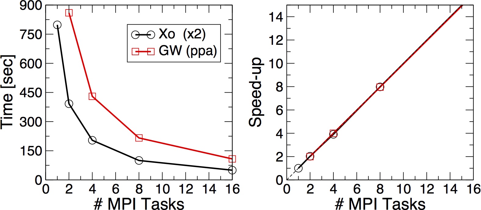
The two numbers (ncpu and tasks-per-node) must match. This time the code should be much faster. Once the run is over try to run the simulation also on 2, 4, 8. Each time please remember to change both the number of tasks per node and the number of CPUs At the end you can try to produce a scaling plot like the following one
Plot the execution time vs the number of MPI tasks and check (do a log plot) how far you are from the ideal linear scaling. To analyze the data you can use the phyton "yambo_parse.py" script which is also provided.
You can use it running
$ ./yambo_parse.py ${jobstring}/r-*
where $jobstring is the string you used for $jobname without the explicit number of MPI tasks.
Advanced: Comparing different parallelization schemes (optional)
Up to now we used the default parallelization scheme. To change this you can open again the job.sh script and modify the section where the yambo input variables are set
X_all_q_CPU= "1 1 $ncpu 1"   # [PARALLEL] CPUs for each role
X_all_q_ROLEs= "q k c v"     # [PARALLEL] CPUs roles (q,k,c,v)
#X_all_q_nCPU_LinAlg_INV= $ncpu   # [PARALLEL] CPUs for Linear Algebra
X_Threads=  0               # [OPENMP/X] Number of threads for response functions
DIP_Threads=  0             # [OPENMP/X] Number of threads for dipoles
SE_CPU= " 1 1 $ncpu"             # [PARALLEL] CPUs for each role
SE_ROLEs= "q qp b"               # [PARALLEL] CPUs roles (q,qp,b)
SE_Threads=  0
In particular "X_all_q_CPU" sets how the MPI Tasks are distributed in the calculation of the parallelization. The possibilities are shown in the "X_all_q_ROLEs"
Pure OpenMP scaling
Next step is instead to check the OpenMP scaling. Set back
ncpu=1
and now use
#SBATCH --tasks-per-node=16

export OMP_NUM_THREADS=16
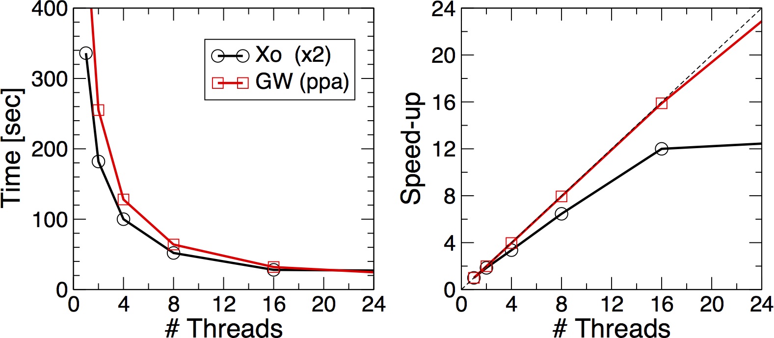
As before the two numbers must match. Try setting OMP_NUM_THREADS to 16, 8, 4 and 2 and again to plot the execution time vs the number of Threads.
MPI vs OpenMP scaling
Which is scaling better ? MPI or OpenMP ? How is the memory distributed ?
Now you can try running simualations with hybrid strategies. Try for example setting:
#SBATCH --tasks-per-node=16
export OMP_NUM_THREADS=4
ncpu=4

