Yambopy tutorial: Yambo databases
In this tutorial we will see some examples on how to read and analyse the data contained in the Yambo netCDF databases, which are not readily available as human readable outputs.
In particular we will take a look at:
- Lattice geometry data (Yambo database:
ns.db1, Yambopy class:YamboLatticeDB). - Dipole matrix elements (Yambo databases:
ndb.dipoles, Yambopy class:YamboDipolesDB). - Exciton energies, symmetries, wavefunctions and spectra (Yambo databases:
ndb.BS_diago_Q*, Yambopy class:YamboExcitonDB).
We will also check the command line instructions to quickly generate yambo SAVE folders.
The scripts of the tutorial, but not the databases, can be found in the yambopy directory:
$cd tutorial/databases_yambopy
The full tutorial, including the Quantum espresso and Yambo databases that we will read, can be downloaded and extracted from the yambo website:
$wget https://media.yambo-code.eu/educational/tutorials/files/databases_yambopy.tar.gz
$tar -xvzf databases_yambopy.tar.gz
$cd databases_yambopy
We will work with monolayer hexagonal boron nitride electron-phonon and exciton data obtained on a 12x12x1 kpoint grid. Beware that these are certainly not converged.
Command line: generating the Yambo SAVE
Yambopy offers a set of command line options. In order to review them, you can type
$yambopy
which will print the output
yambopy v0.7
Available commands are:

      plotem1s ->     Plot em1s calculation.
    analysebse ->     Study the convergence of BSE calculations.
     analysegw ->     Study the convergence of GW calculations by looking at the change in band-gap value.
  plotexcitons ->     Plot excitons calculation.
         addqp ->     Add corrections from QP databases.
       mergeqp ->     Merge QP databases.
          save ->     Produce a SAVE folder.
          gkkp ->     Produce a SAVE folder including elph_gkkp databases.
         bands ->     Script to produce band structure data and visualization from QE.
        serial ->     Script to update serial numbers of yambo ndb.* databases in order to import them to new calculations.
    gwsubspace ->     Script to calculate off-diago corrections of yambo ndb.QP databases in order to plot band structure.
         phinp ->     Script to update the explicit list of q-points in a ph input file (ldisp=.false., qplot=.true.).
       convert ->     Script to convert RL number in Ry energy units using ndb.gops.
       bsesize ->     Script to calculate the expected BSE kernel size, in GB, to be loaded by each MPI task.
           l2y ->     Calculate gauge-invariant electron-phonon matrix elements with LetzElPhC and convert them into Yambo format.
     exc-irrep ->     Script to get the irreducible representation labels for excitonic states. [-h for help]
        exc-wf ->     Real space exciton wf for either fixed hole/electron. [-h for help]
      exc-sort ->     Script to sort excitonic states according to energies and intensities. [-h for help]
For this tutorial, we will need the save and gkkp options.
By typing in one of these, additional information about how to run the commands will be printed, e.g.:
$yambopy save

Produce a SAVE folder

Arguments are:
  -nscf, --nscf_dir  -> Path to nscf save folder
  -y, --yambo_dir    -> <Optional> Path to yambo executables
The quantum espresso save for hBN is provided in the directory BSE_saves/QE_saves/hBN.save (you can check the contents of the various folders).
Then, following the instructions printed on screen, we can generate a yambo SAVE from the hBN.save by typing
$yambopy save -nscf BSE_saves/QE_saves/hBN.save
This should produce a SAVE folder in the current directory.
Lattice intro: plot k-point coordinates in IBZ/BZ
For this section we will use the script bz_plot.py.
By inspecting the SAVE folder we have just generated, we will find the ns.db1 database which contains all the geometry and lattice information.
We are now going to read it in python by using the Yambopy class YamboLatticeDB, which can be instanced like this:
from yambopy import YamboLatticeDB
ylat = YamboLatticeDB.from_db_file(filename="PATH/TO/SAVE/ns.db1")
(remember to edit the variable save_path in order to point at your yambo SAVE).
The ylat object now contains many useful information as attributes, such as the k-points in Cartesian or crystal coordinates, the system symmetries, lattice constants and basis vectors in real and reciprocal space, etc.
The k-points are also automatically expanded in the full Brillouin zone from the irreducible one (you can turn this off with the option Expand=False).
Directly printing the object with
print(ylat)
will also give us some general parameters related to the database.
Now check the bz_plot.py script. You will see that it performs three plots:
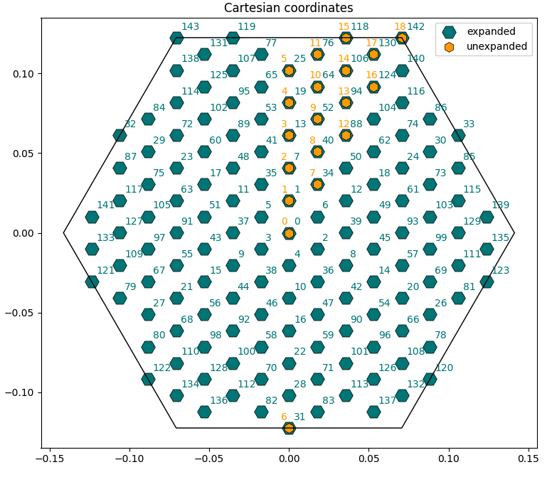
- Scatterplot of the k-points in Cartesian coordinates with both expanded and unexpanded grids, with annotated indices [
Cartesian_Plot=True]. - Scatterplot of the k-points in crystal coordinates [
Crystal_Plot=True]. - Manual transformation of a chosen k-point from irreducible to full Brillouin zone (you can change the index
i_kin the script to check different cases) [Symmetry_Plot=True].
Below, the result of the first plot.
What about the units?
Below we report the relation between units used in Yambo, Quantum Espresso, and Yambopy.
- bohr^-1 (atomic units):
YamboLatticeDB.car_kpoints*2.*pi. Divide by the bohr-to-angstrom conversion factor to obtain angs^-1 - Yambo cartesian units (
[cc]in Yambo outputs):YamboLatticeDB.car_kpoints*2.*pi(same as above). - QE cartesian units (
[cart. coord. in units 2pi/alat]in QE outputs):YamboLatticeDB.car_kpoints*YamboLatticeDB.alat[0]. - Internal yambo units (
[iku]in yambo outputs):YamboLatticeDB.iku_kpoints - Fractional coordinates (
[rlu]in yambo,cryst. coord.in QE):YamboLatticeDB.red_kpoints.
Dipoles intro: plots of dipoles on BZ, plot of IP absorption
In this section we will use the script dipoles_plot.py and read the dipole databases generated in an optical absorption calculation by yambo. Keep in mind that from now on we will use the "BSE" yambo SAVE generated in the first section.
The databases written after a calculation of optical properties with yambo (dipoles, static screening, excitons) are in the directory BSE_saves/BSE_databases. Here we will also find ndb.dipoles which is needed now, since it contains the matrix elements d_{vck}(\alpha) where vk and ck are the valence and electron states involved in the transition and \alpha the polarisation direction of the external electric field.
In order to read it in python we use the Yambopy class YamboDipolesDB, which can be instanced like this:
ydip = YamboDipolesDB(ylat,save='path/to/BSE/databases',filename='ndb.dipoles')
(notice that it requires a previous instance of YamboLatticeDB).
In addition, in order to read the Kohn-Sham energies, we can also instance the YamboElectronsDB as
yel = YamboElectronsDB.from_db_file(folder='path/to/SAVE')
The object ydip now has a method that permits to retrieve the independent-particle absorption spectrum with customly chosen energy range, steps, and broadening:
w, eps2 = ydip.ip_eps2(yel)
In order to see all this in action, take a look at the dipoles_plot.py script. You will see that it performs two plots:
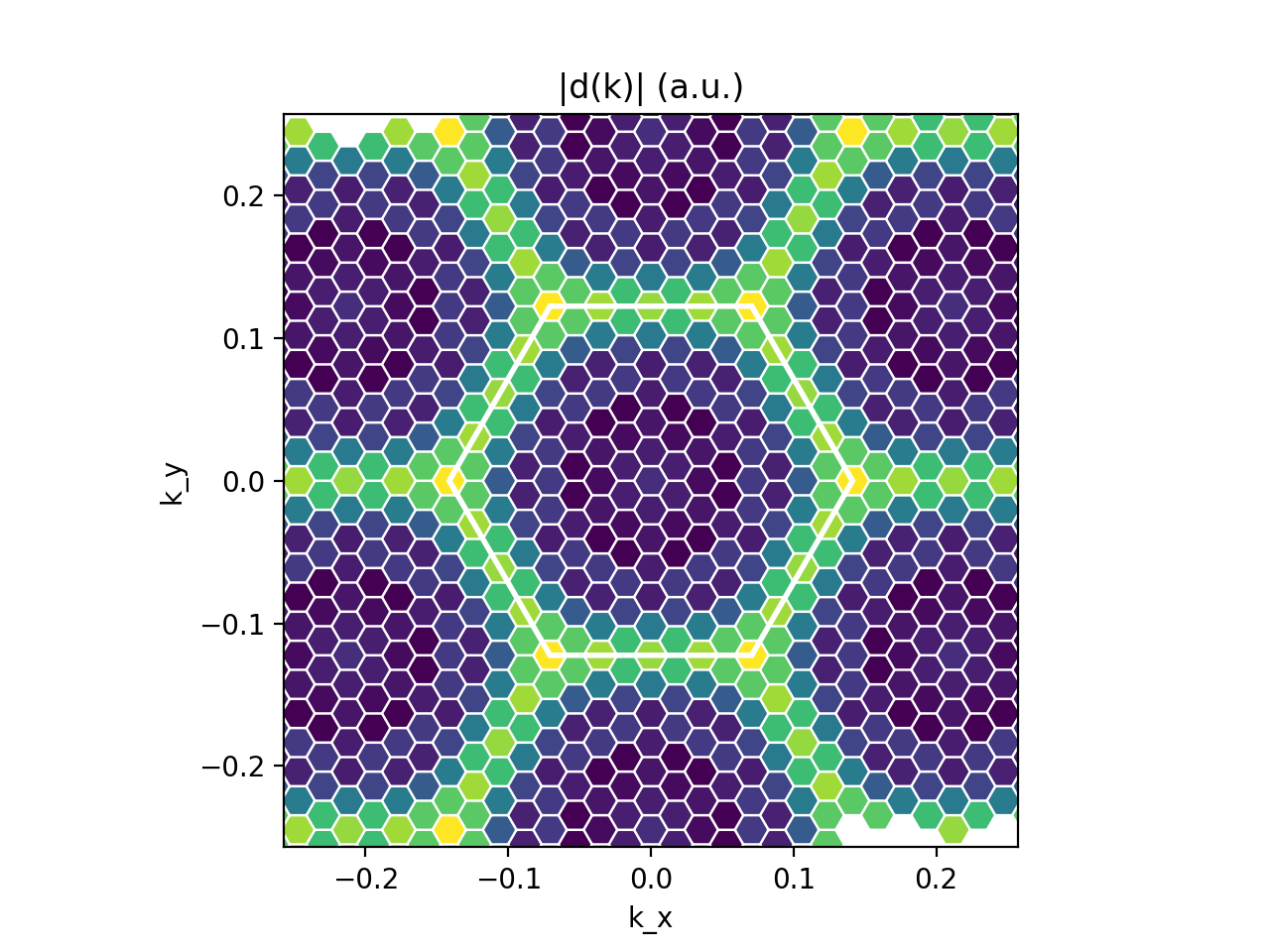
- Plot of |d(k)| in the BZ for selected v,c and \alpha (we choose the layer plane 'xy') [
Kspace_Plot=True]. From this plot you can appreciate which sections of the BZ contribute the most to the absorption rate. - Plot of the independent-particles absorption spectrum [
Absorption_Plot=True].
You can play with the indices and the plot parameters to check what happens.
Exciton intro 1: read and sort data
In this section we will use both the script exc_read.py and the command line in order to read the exciton data resulting from a BSE calculation to familiarise with their structure. This time we are going to read the ndb.BS_diago_Q* databases which correspond to BSE calculations at various momenta Q (Q=1 being the zero-momentum optical absorption limit - notice that python indexing starts from 0, while the databases are counted starting from 1).
In order to read them in python we use the Yambopy class YamboExcitonDB, which can be instanced like this:
yexc = YamboExcitonDB.from_db_file(ylat,filename=f'path/to/BSE/databases/ndb.BS_diago_Q{i}')
(where i is the number of BS_diago_Qi file. Notice that it requires a previous instance of YamboLatticeDB).
Now the yexc object contains information about the exciton energies (yexc.eigenvalues), wave functions (yexc.eigenvectors) and intensities (yexc.l_residuals, yexc.r_residuals) for Qpoint i_Q. You can start by keeping Q1 which is the optical limit and then check other momenta.
The exciton wave function components A_{vck}^{\lambda Q} (\lambda being the exciton index) are stored as A_{t}^{\lambda} in each Q-dependent database, with t being the transition index grouping the single-particle indices vck. Therefore, yexc.eigenvectors is an array with (N_excitons,N_transitions) dimension. In order to make the connection t->kcv, the table yexc.table provides k,v,c and spin indices corresponding to each transition.
In order to get a clearer picture, take a look at the script exc_read.py. Run it and try to understand the outputs.
$ python exc_read.py
Actually, we can produce output files with the sorted exciton energies in a much more convenient way by using the command line instruction exc-sort. Check its syntax via:
$ yambopy exc-sort -h
Then, we run it for our specific calculation with:
$ yambopy exc-sort --save BSE_saves/YAMBO_saves/SAVE -J BSE_saves/BSE_databases --iqpt 1
Recall that that the path given to --save must be the directory that contains the ns.db1 yambo database (usually called... SAVE). The path given to -J must be the directory that contains the results of the BSE calculation, namely the ndb.BS_diago_Q1 file. The final argument is the center-of-mass momentum of the exciton. In a standard absorption calculation, you only need the first Q-point which describes vertical electronic transitions. However, if you calculate the exciton dispersion, you will produce a ndb.BS_diago_QN at each momentum index N that you selected for the yambo BSE calculation.
This command should produce the o-BSE_databases.exc_qpt1_sorted_E.dat and o-BSE_databases.exc_qpt1_sorted_I.dat output files for you to inspect. These are very useful as they allow for identification of degenerate states and degree of optical activity. You will see that in our system most states are doubly degenerate, a byproduct of crystal symmetry. This is an updated version of the ypp exciton analysis that you can find here.
Exciton intro 2: symmetry analysis and wavefunction plot in real space
Symmetries of excitons
We can analyse the symmetries of the excitonic wavefunctions in terms of irreducible representation of the point group of the system (if at Q=0) or the Q little group. For more information, the methodology is explained in Ref. [1].
We use the exc-irrep command line option, check the arguments with:
$ yambopy exc-irrep -h
We know from the previous section (by inspecting the sorted energies) that the first four BSE eigenvalues correspond to two doubly-degenerate bright states. Let us analyse their symmetry by running
$ yambopy exc-irrep --path BSE_saves/YAMBO_saves -J BSE_saves/BSE_databases --iqpt 1 --nstates 4
This command first loads the electronic wave functions and calculated the electronic representation matrices (called Dmats in the code). As a second step, they are used to compute the excitonic representation matrices.
We obtain the following output:
========================================
Group theory analysis for Q point : (0.000000, 0.000000, 0.000000)
****************************************
Little group :  D3h
Little group symmetries :  [ 1  2  3  4  5  6  7  8  9 10 11 12]
Classes (symmetry indices in each class):
               E    :  [1]
            2S_3    :  [2 6]
            2C_3    :  [3 5]
         sigma_h    :  [4]
            3C_2    :  [ 7  9 11]
        3sigma_v    :  [ 8 10 12]

====== Exciton representations ======
Energy (eV),  degeneracy  : representation
----------------------------------------
1.9139                2  :  E'
2.5988                2  :  E'
****************************************
This is similar to the group theory analysis done by Quantum Espresso on the electronic states, and is actually analogous to the one performed for the phonon modes of crystals. We see that the first two states transform as the E' representation of the D3h point group of the crystal. By optical selection rules, only states with this symmetry can form absorption peaks in monolayer BN when light is polarized along the layer plane.
We could go further and calculate the total crystal angular momentum of these states, while also rotate the degenerate exciton states so that they are both eigenvectors of the BSE Hamiltonian and the total crystal angular momentum operator. This is very useful for analyses involving selection rules, exciton-boson couplings, chirality, etc. This is an advanced topic and will not be covered, nonetheless an example script is provided in the tutorial folder called total_crystal_angular_momentum_exciton.py.
What to do when symmetry analysis does not seem to work well
- Check for warnings during execution. If the BSE calculation was done with a response function that breaks the symmetries (such as the longitudinal response in place of the transverse one at q=0), that may explain the issues.
- If the exciton density of states is very high (such as for a bulk 3D system or for a 2D system at higher energies in the optical spectrum), the analyser may fail to resolve degenerate states, and incorporate a bunch of states together. The symmetry analysis will still be performed but the representation labels will appear as summed. In severe cases, the code may crash. You can try to get a better result by carefully selecting the degeneracy tolerance with
degen_toland restricting the number of states withnstatesin the command line options.
Exciton wave functions in real space
We can also plot the wave functions of the exciton states on the crystal lattice. In practice, what we do is set the position of the hole at a "physical" point, and then visualize the resulting electronic distribution:
[math]\displaystyle{ I^{e}_{\lambda \mathbf{Q}}(\mathbf{r}_e)= |\Psi_{\alpha \mathbf{Q}}(\mathbf{r}_e,\mathbf{r}_h=\mathbf{r}_0)|^2 }[/math]
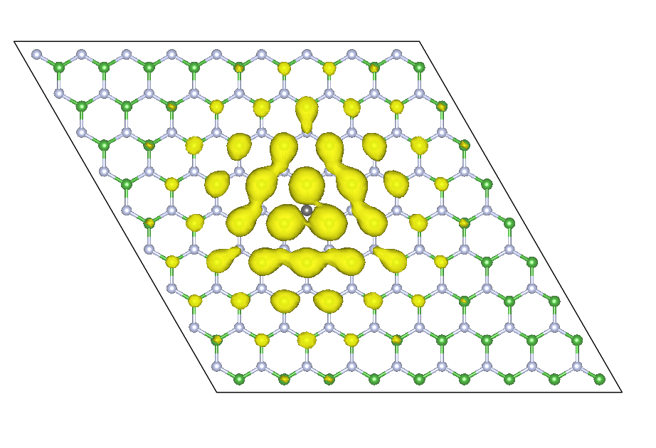
Let us focus on the lowest exciton state, which gives rise to the largest peak in absorption (see the last part of the tutorial). We will set the hole position on top of a nitrogen atom, since that's where the [math]\displaystyle{ p_z }[/math] orbitals where the hole comes from are mostly localized.
If we don't know the correct coordinates, we can modify the bz_plot.py script by adding (after instancing the lattice object):
for iat in range(len(ylat.atomic_numbers)): print(ylat.atomic_numbers[iat],ylat.red_atomic_positions[iat])
which will print
5 [0.6666667 0.3333333 0.       ]
7 [-0.6666667 -0.3333333  0.       ]
In order to make the plot, we have to give yambopy the same inputs that are used in the equivalent ypp calculation. First, let's check all the options via
$ yambopy exc-wf -h
Then, we can run our calculation (by selecting a 9x9x1 supercell and a 30 Ry cutoff) as
$ yambopy exc-wf --path BSE_saves/YAMBO_saves -J BSE_saves/BSE_databases --iqpt 1 --iexe 1 --supercell 9 9 1 --wfc_cutoff 30 --hole 0.33333333 0.66666667 0.03
Yambopy will produce a *.cube file that can be visualized with VESTA, xcrysden or the like, producing a figure similar to the one below.
The example script exc_real_wf.py, which runs the same calculation by explicitly calling the necessary functions, will give you more info about what is happening behind the scenes.
We see that electron is localised in [math]\displaystyle{ p_z }[/math]-like distributions on top of boron atoms around the nitrogen where the hole is set.
Exciton intro 3: plot exciton weights on k-BZ and (interpolated) band structure
In this section we will use the script exc_kspace_plot.py and work with the quantities defined in the previous section.
For now, only the i_Q=0 case is implemented in this section. We want to check the relative importance of the various (vk->ck) electronic transitions in forming a certain excitonic state.
Since many excitonic states are degenerate, we first need to tell Yambopy which states we want to check. For example, in monolayer hexagonal boron nitride, the lowest-bound exciton - forming the main peak in the BSE absorption spectrum - is doubly degenerate. In order to analyse it, in the exc_kspace_plot.py script we set
states = [1,2]
(we can also set [3,4] to check the second excitonic state, and then [5] for the non-degenerate third state, and so on; we can check degeneracies by printing the energies using the script exc_read.py).
In order to make a band structure plot, it is necessary to read the band energies, for example with the YamboSaveDB class
yel = YamboSaveDB.from_db_file(folder='path/to/SAVE')
and specify the path in the BZ using crystal coordinates via the Path function:
npoints = 20
path = Path([ [[  0.0,  0.0,  0.0],'$\Gamma$'],
              [[  0.5,  0.0,  0.0],'M'],
              [[1./3.,1./3.,  0.0],'K'],
              [[  0.0,  0.0,  0.0],'$\Gamma$']],
              [int(npoints*2),int(npoints),int(sqrt(5)*npoints)] )
Now let's take a closer look at the exc_kspace_plot.py script. You will see that it performs three plots:
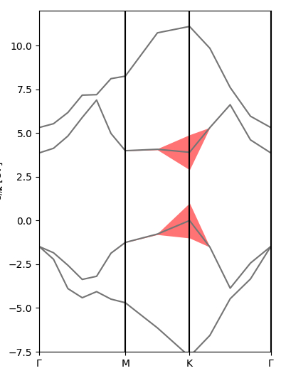
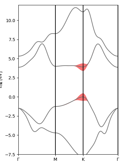
- Plot of |A(k)| in the k-BZ for the selected exciton state. You can see how most contributions come from the area around K and the MK direction [
Kspace_Plot=True]. - Plot of |A(v,c,k)| on the electronic band structure for the selected exciton state. Here you can better see how the top valence and bottom conduction around MK are mostly involved [
Bands_Plot=True]. - Plot of interpolated |A(v,c,k)| on the interpolated electronic band structure for the selected exciton state [
Bands_Plot_Interpolated=True].
As always, try to play with the parameters, for example by changing the excitonic states to analyse.
Exciton intro 4: plot BSE optical absorption with custom options
In this section we will use the script exc_abs_plot.py and work with the quantities defined in the previous sections.
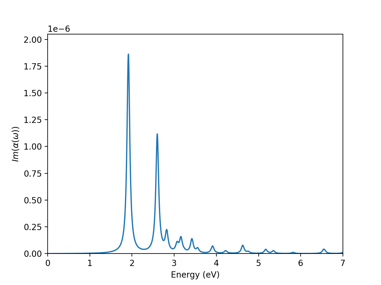
The class YamboExcitonDB also enables us, of course, to read the dielectric function eps(w) and print absorption and related spectra in python.
The advantages over using the standard human-readable yambo outputs are mainly two:
- We can freely select energy ranges, energy steps, peak broadenings and number of excitonic states included without having to rerun the
yamboexecutable every time. This reduces the chance of mistakenly editing the yambo input and allows for greater freedom since these plots can now be done in your local machine without having to transfer the output data from a remote cluster. - The dielectric function constructed from netCDF database variables has a much higher precision (number of significant digits) than the human readable output, which may be important if you want to perform additional operations in python (e.g., computing refractive index, reflectivity and other optical spectra from it, performing finite-difference derivatives, etc).
We can read eps(w) as a numpy array with the specified options as (energy values are in eV):
w, eps = yexc.get_chi(nexcitons='all',emin=0,emax=7,estep=0.005,broad=0.04)
Or, you can directly prepare a plot of its imaginary part with
w, chi = yexc.plot_chi_ax(ax,nexcitons='all',emin=0,emax=7,estep=0.005,broad=0.04)
where ax is a previously defined Axes object from matplotlib.
In order to see how this works, let's take a look at the exc_abs_plot.py script.
You will see that it performs the two operations described above:
- Plotting the BSE absorption spectrum [
Absorption_Plot=True]. - Reading the complex dielectric function.
Try to customise the plots by changing the nexcitons, emin, emax, estep, broad parameters.
Links
- Back to Rome 2023#Tutorials
- Back to ICTP 2022#Tutorials
References
- ↑ Symmetries of excitons, M. Nalabothula et al., preprint arXiv
