Modena 2025 : Yambopy part 2
In this tutorial we will first plot and interpolate GW band structures calculated with YAMBO, then deal with the analysis of excitons from a BSE calculation.
Make sure you have completed Modena 2025: Yambopy part 1 and have the relevant databases in your $SCRATCH directory.
cd $SCRATCH
cd YAMBOPY_TUTORIALS
GW calculations
Tutorial 1: GW bands
Yambopy can be used either to run Yambo and QE calculations, or to analyse the results of QE and Yambo by dealing with their generated databases. This is done with a variety of classes included in the qepy (for QE) or yambopy (for Yambo) modules. In the case of Yambo GW quasi-particle calculations, we can use the yambopy class YamboQPDB to read the database produced by the simulation. Enter in the folder
cd databases_qepy/gw-bands
We can use this to find the scissor operator, plot the GW bands and to interpolate the GW bands on a smoother k-path. The example runs by typing:
python plot-qp.py
See below for an explanation of the tutorial. As usual, we can import the qepy and yambopy libraries:
 from yambopy import YamboLatticeDB,YamboQPDB
 from qepy import Path
We define the k-points path.
 npoints = 10
 path = Path([ [[  0.0,  0.0,  0.0],'$\Gamma$'],
               [[  0.5,  0.0,  0.0],'M'],
               [[1./3.,1./3.,  0.0],'K'],
               [[  0.0,  0.0,  0.0],'$\Gamma$']], [int(npoints*2),int(npoints),int(sqrt(5)*npoints)] )
Importantly, the number of points is a free choice used only in case of interpolation. We can increase the variable npoints as we wish, it just means that the interpolation step will take more time. In order to analyse GW results we need to have the file related to the basic data of our Yambo calculation (SAVE/ns.db1) and the netcdf file with the quasi-particle results (ndb.QP). We load the data calling the respective classes:
# Read Lattice information from SAVE
lat  = YamboSaveDB.from_db_file(folder='SAVE',filename='ns.db1')
# Read QP database
ydb  = YamboQPDB.from_db(filename='ndb.QP',folder='qp-gw')
(as you know by now, in the yambopy module each class is specialised to read a specific Yambo database)
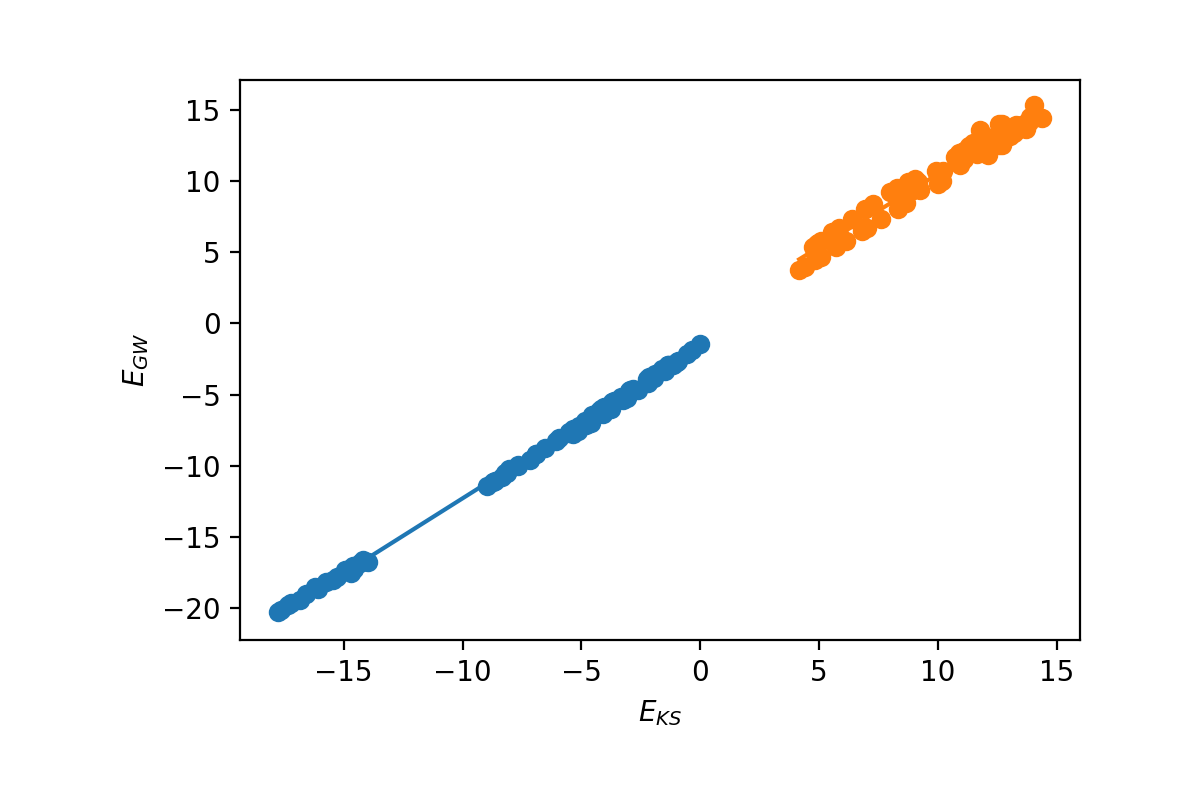
The first option is to plot the energies and calculate the ideal Kohn-Sham to GW scissor operator. We need to select the index of the top valence band:
n_top_vb = 4
ydb.plot_scissor_ax(ax,n_top_vb)
Yambopy displays the fitting and also the data of the slope of each fitting. Notice that this is also a test if the GW calculations are running well. If the dependence is not approaching linear you should double-check your results!
In this case the slope is:
valence bands:
slope:     1.0515886598785766
conduction bands:
slope:     1.026524081134514
scissor list (shift,c,v) [eV,adim,adim]: [1.8985204833551723, 1.026524081134514, 1.0515886598785766]
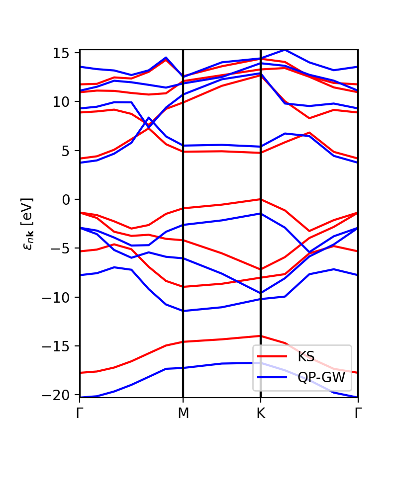
In addition to the scissor operator, we can plot the GW (and DFT) band structure along the path. The first choice would be to plot the actual GW calculations, without interpolation, to check that the results are meaningful (or not). This plot is independent of the number of k-points (npoints) that we want to put in the interpolation. The class YamboQPDB finds the calculated points that belong to the path and plots them. Be aware that if we use coarse grids the class would not find any point and the function will not work.
ks_bs_0, qp_bs_0 = ydb.get_bs_path(lat,path)
ks_bs_0.plot_ax(ax,legend=True,c_bands='r',label='KS')
qp_bs_0.plot_ax(ax,legend=True,c_bands='b',label='QP-GW')
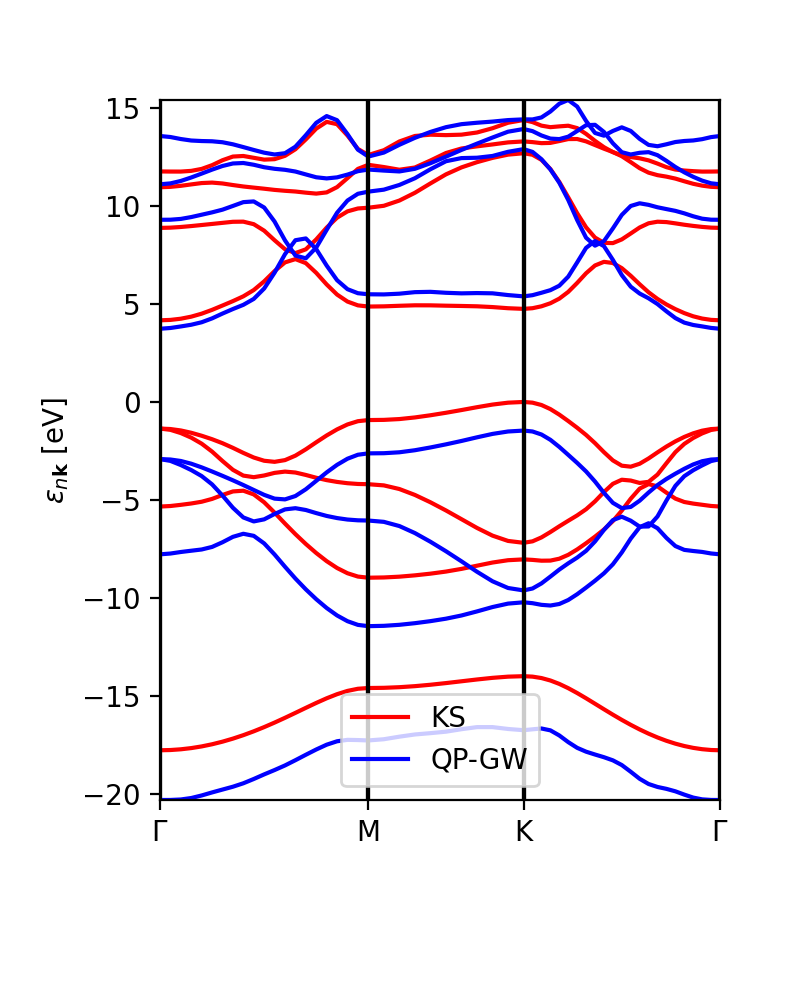
The interpolation of the DFT and GW band structures looks similar:
ks_bs, qp_bs = ydb.interpolate(lat,path,what='QP+KS',lpratio=20)
ks_bs.plot_ax(ax,legend=True,c_bands='r',label='KS')
qp_bs.plot_ax(ax,legend=True,c_bands='b',label='QP-GW')
The lpratio can be increased if the interpolation does not work as well as intended. The SKW interpolation scheme is the same one implemented in abipy (the python interface for the Abinit DFT code).
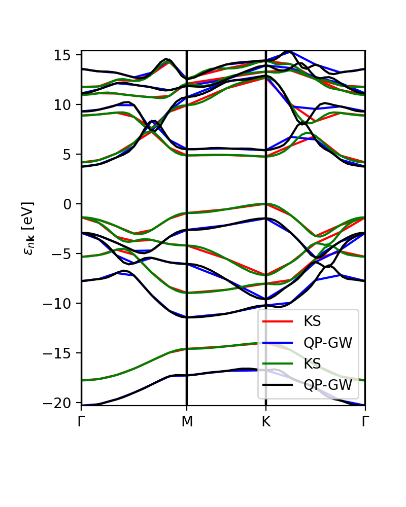
Finally, we can compare the calculated GW eigenvalues with the interpolation.
Excitons
ciao
Links
- Back to Modena 2025 : Yambopy part 1
- Back to Modena 2025


