Dielectric function from Bloch-states dynamics (5.3)
Step 0: Theoretical background
The dynamics of Bloch-states is found by integrating a set of Time Dependent Effective Schrödinger Equations (TD-ESEs). Effective means that an effective Hamiltonian is considered. We consider the many-body effective Hamiltonians seen in the Linear response from real time simulations. In addition, one can also consider effective Hamiltonians based on density-functional theory. The latter choice gives time-dependent density-functional theory.
The coupling between electrons and the external field is described by means of the Modern Theory of Polarization:
Where [math]\displaystyle{ | v_{i \mathbf{k}} \rangle }[/math] are the time-dependent Bloch states (corresponding to the filled Bloch-states at zero-field), [math]\displaystyle{ \mathcal E(t) }[/math] is the external field and the term [math]\displaystyle{ i e \partial k }[/math] is the dipole operator consistent with periodic boundary condition. For more details on this last term, see Ref. [1] and [2].
[math]\displaystyle{ h_{rt} }[/math] is the Hamiltonian,
.
This contains the equilibrium Hamiltonian, that is the zero-field eigenvalues evaluated through DFT; the quasiparticle corrections, evaluated from GW or estimated from experiment, and the variation of the self-energy. The latter is a functional of the density matrix [math]\displaystyle{ \rho }[/math], which is obtained from the Bloch states.
From the solution of the equation of motion for the Bloch states, the polarization is calculated by means of Berry's phase
.
One can decide the level of theory by selecting the terms to include in the Hamiltonian:
- by including only the first term, one selects the independent-particle approximation
- by including the first and second terms, one selects the independent-quasiparticle approximation
- by including the first, second terms and the Hartree part of the self-energy, one selects the time-dependent Hartree or random-phase approximation
- by including all terms, one selects the time-dependent Screened-exchange or Bethe-Salpeter equation level of theory.
The type of "experiment" to perform, or of the response one would like to extract, depend on the time-dependent field in input and the post-processing of the Berry's phase polarization. The induced polarization is the sum of the responses of the system to all orders in the external field: [math]\displaystyle{ \bf{P}(t) = \sum_{n=-\infty}^{+\infty} \bf{P}_n (t) }[/math]
In the case we are interested in linear response only, we use a delta-like electric field that excites all frequencies of the system. We choose the intensity of the field [math]\displaystyle{ E }[/math] to be weak enough so that the response is dominated by the first order term. The response at all frequencies is obtained by taking the Fourier-transform of the polarization as
[math]\displaystyle{ \chi(\omega) = \frac{P(\omega)}{E} }[/math].
The response [math]\displaystyle{ \chi }[/math] is related to the dielectric function through the relation [math]\displaystyle{ \epsilon(\omega) = 1 + 4 \pi \chi(\omega) }[/math]. See also Ref. [2].
Notes:
- Length vs Velocity gauge: the equations of motion of Yambo are in the length gauge. Other codes choose instead to work in the velocity gauge. If you want to know more about the advantages and disadvantages of the two gauges read section 2.7 of Ref. [3].
- Advantages and disadvantages with respect to the density-matrix based formalism: Yambo implements two distinct formalisms for studying the real-time response, the one based on density-matrix and the one based on Boch states. Which formalism is best to use depends on what one wants to simulate. The dynamics formulation in terms of density matrix or non-equilibrium Green's functions allows a systematic treatment of correlation effects and electron-phonon coupling[4], but the price to pay is that the coupling with the external field is correct only to the linear order. This formalism is important in all those phenomena where electronic relaxation plays a major role. On the other hand, the formulation in terms of the Bloch states treats coupling with the external field in an exact way even beyond the linear regime, and for this reason, it allows the description of phenomena coherent with the external fields and to access, for example, non-linear responses.
Step 1: Prerequisites
In this example, we will consider a single layer of hexagonal boron nitride (hBN). Before running real time simulations in yambo you need to:
- download input files and Yambo databases for this tutorial here: hBN-2D-RT.tar.gz.
- perform the steps described in Prerequisites for Real Time propagation with Yambo (5.3).
Step 2: Independent-particle approximation
Similar to what you have seen in the tutorial for the density matrix formalism (Real time approach to linear response) we start from the lowest level of theory. Here it is assumed you ran the tutorial on the density-matrix formalism and so you are familiar with the optical spectrum of 2D h-BN at this level of theory. You will recognise that the input and output for the Bloch-state formalism are very similar to those for the density-matrix formalism.
Run the simulations
You should now be inside the folder YAMBO_TUTORIALS/hBN-2D-RT/YAMBO/FixSymm.
First of all, create a directory for the inputs to be run by yambo_nl:
mkdir Inputs_nl
Then, use the command:
yambo_nl -nl n -F Inputs_nl/01_td_ip.in
to generate the input (OMP, angular and extra fields keywords are omitted for brevity):
nloptics                         # [R] Non-linear spectroscopy
% NLBands
  3 | 6  |                           # [NL] Bands range
%
NLverbosity= "high"              # [NL] Verbosity level (low | high)
NLtime= 55.000000           fs    # [NL] Simulation Time
NLintegrator= "INVINT"           # [NL] Integrator ("EULEREXP/RK2/RK4/RK2EXP/HEUN/INVINT/CRANKNIC")
NLCorrelation= "IPA"             # [NL] Correlation ("IPA/HARTREE/TDDFT/LRC/LRW/JGM/SEX")
NLLrcAlpha= 0.000000             # [NL] Long Range Correction
% NLEnRange
 -1.000000 |-1.000000 |      eV    # [NL] Energy range
%
NLEnSteps= 1                     # [NL] Energy steps
NLDamping= 0.000000        eV    # [NL] Damping (or dephasing)
RADLifeTime=-1.000000      fs    # [RT] Radiative life-time (if negative Yambo sets it equal to Phase_LifeTime in NL)
#EvalCurrent                   # [NL] Evaluate the current
#FrPolPerdic                   # [DIP] Force periodicity of polarization respect to the external field
HARRLvcs= 18475            RL    # [HA] Hartree     RL components
EXXRLvcs= 18475            RL    # [XX] Exchange    RL components
% Field1_Freq
 0.100000 | 0.100000 |         eV    # [RT Field1] Frequency
%
Field1_NFreqs= 1                 # [RT Field1] Frequency
Field1_Int=  1000.00       kWLm2 # [RT Field1] Intensity
Field1_Width= 0.000000     fs    # [RT Field1] Width
Field1_kind= "DELTA"           # [RT Field1] Kind(SIN|COS|RES|ANTIRES|GAUSS|DELTA|QSSIN)
Field1_pol= "linear"             # [RT Field1] Pol(linear|circular)
% Field1_Dir
 0.000000 | 1.000000 | 0.000000 |        # [RT Field1] Versor
%
Field1_Tstart= 0.010000    fs    # [RT Field1] Initial Time
Note that the standard input of yambo_nl has default settings for nonlinear response (e.g. the SOFTSIN for the Field1_kind (that set the time-dependence 'kind' of the field).
Set the field direction Field1_Dir along y, the field kind to DELTA, the length of the simulation NLtime to 55 fs, select the bands from 3 to 6 (NLBands) and set the NLDamping to zero. The fields you need to change with respect to the default settings are shown above in red.
Now run
yambo_nl -F Inputs_nl/01_td_ip.in -J TD-IP_nl -C TD-IP_nl &
and then monitor the progress with
 tail -f TD-IP_nl/o-TD-IP_nl.polarization_F1
 ctrl+C
The code produces different files (in the TD-IP_nl directory, all with the suffix TD-IP_nl: o-TD-IP_nl.polarization_F1 that contains the polarization, o-TD-IP_nl.external_potential_F1 the external field we used, and finally r-TD-IP_nl_nloptics a report with all information about the simulation.
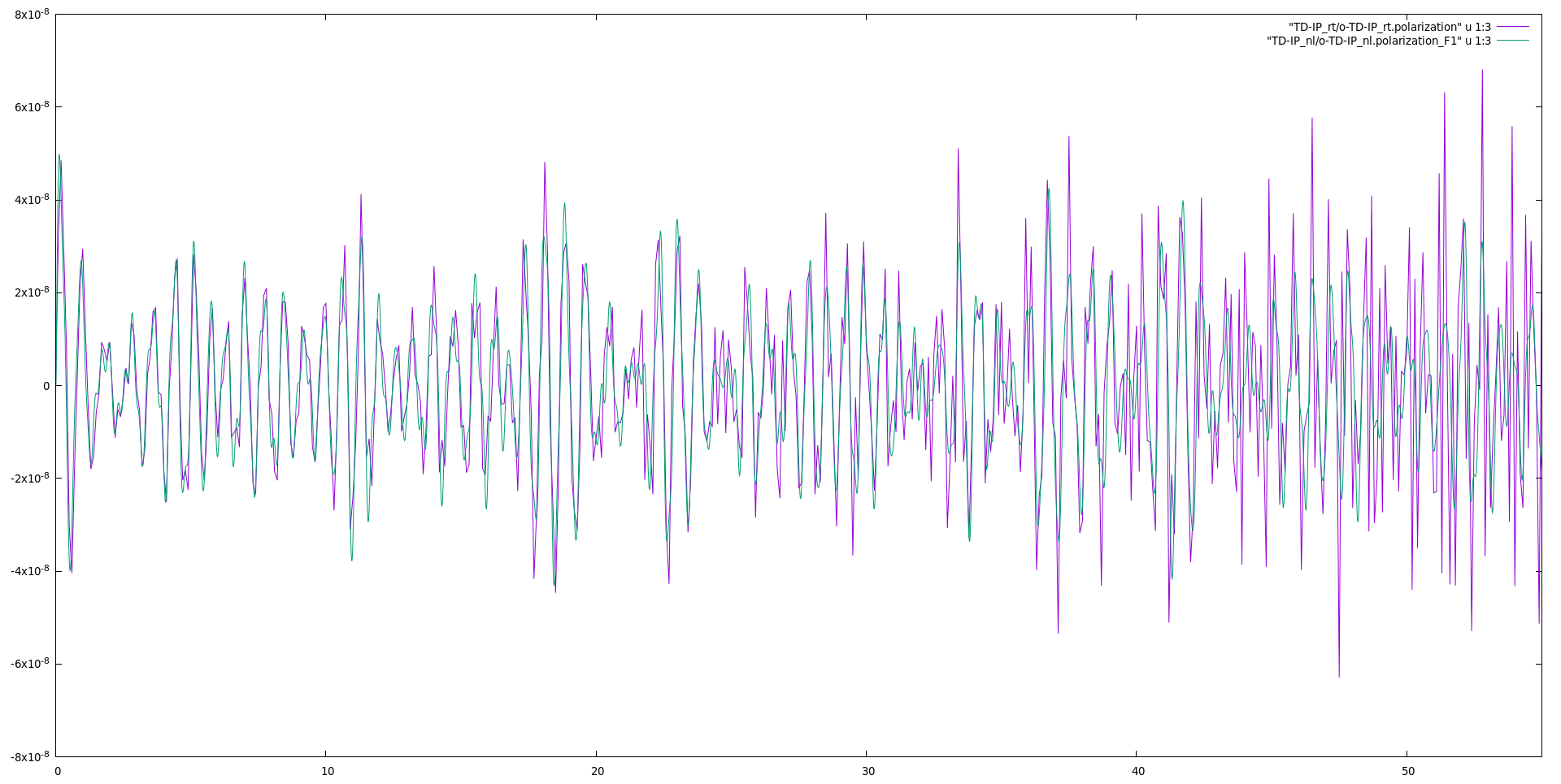
Plot the third column of o-TD-IP_nl.polarization_F1 versus the first one (time-variable) to get the time-dependent polarization along the y-direction:
gnuplot> p 'TD-IP_nl/o-TD-IP_nl.polarization_F1' u 1:3 w l
Output postprocessing: the dielectric function
Once we obtained the polarization, we Fourier transform the polarization to obtain the dielectric function.
Use the command:
ypp_nl -nl -F Inputs_nl/02_ypp_abs.in
to generate the input file:
nonlinear                    # [R] NonLinear Optics Post-Processing
Xorder= 1                    # Max order of the response functions
% TimeRange
-1.000000 |-1.000000 | fs    # Time-window where processing is done
%
ETStpsRt= 1001                # Total Energy steps
% EnRngeRt
  0.00000 | 10.00000 | eV    # Energy range
%
DampMode= "LORENTZIAN"             # Damping type ( NONE | LORENTZIAN | GAUSSIAN )
DampFactor=  0.10000   eV    # Damping parameter
where we set a Lorentzian smearing corresponding to 0.1 eV. Note that due to the finite time of our simulation, we need to introduce a finite smearing to Fourier transform the result.
To run the post-processing, use the command:
ypp_nl -F Inputs_nl/02_ypp_abs.in -J TD-IP_nl -C TD-IP_nl
and obtain the files for the dielectric constant along with the field direction, the EELS along with the same direction, and the damped polarization.
o-TD-IP_nl.YPP-eps_along_E
o-TD-IP_nl.YPP-eels_along_E
o-TD-IP_nl.YPP-damped_polarization
inside the folder TD-IP_nl
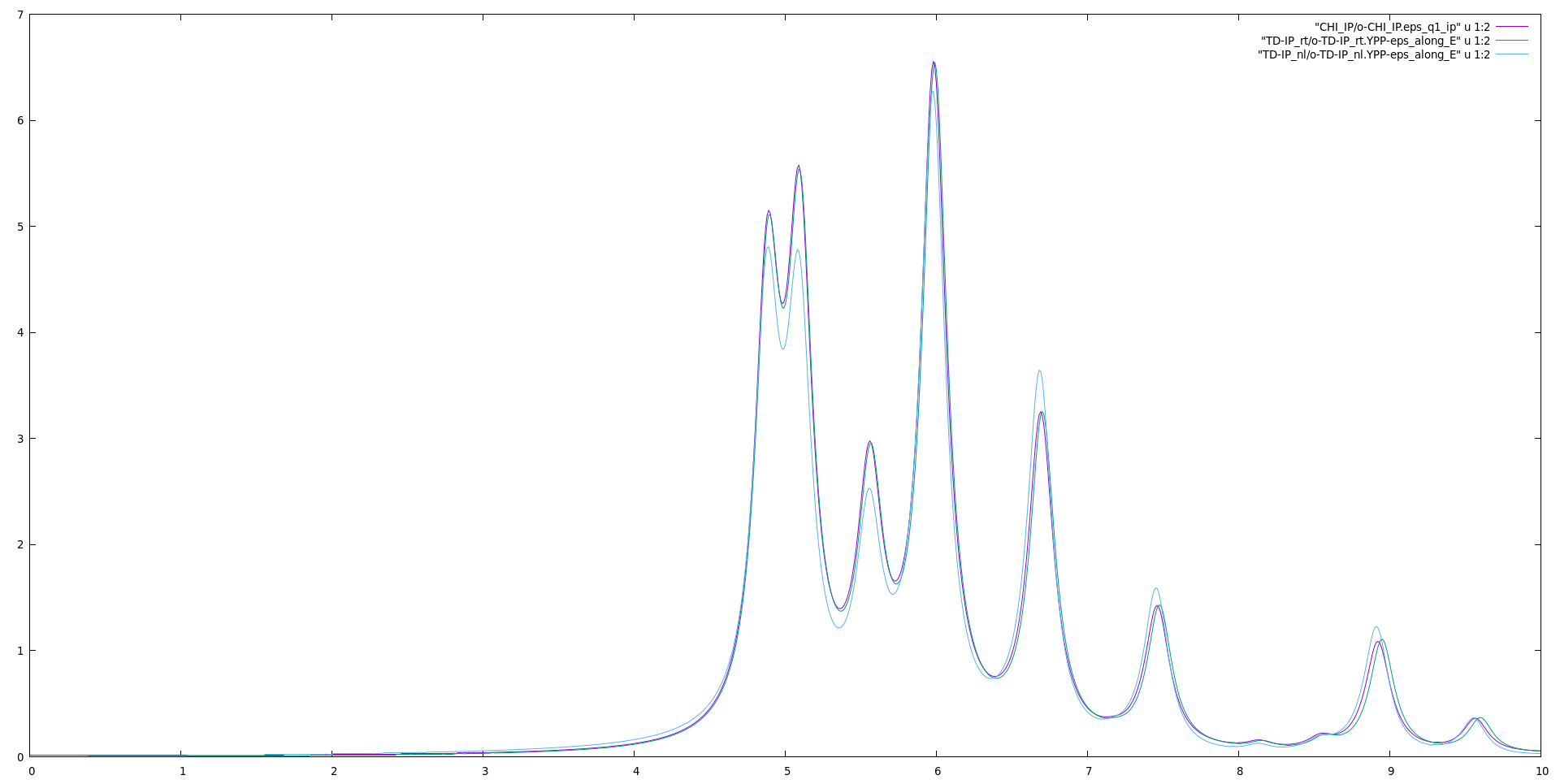
Plot the dielectric constant and compare it with the linear response and the density-matrix formalism (available from the Real time approach to linear response tutorial):
gnuplot
plot "../CHI_IP/o-CHI_IP.eps_q1_ip" u 1:2 w l
rep "TD-IP_nl/o-TD-IP_nl.YPP-eps_along_E" u 1:2 w l
The differences observed with the spectra obtained from the linear-response formalisms are due to how the dipoles are evaluated. Within the linear-response formalism, dipoles are computed as [math]\displaystyle{ \frac{1}{E_{c \mathbf{k}}-E_{v \mathbf{k}}} \left\langle v \mathbf{k}\left|\mathbf{p}_{\alpha}+\mathrm i\left[V^{\mathrm{NL}}, \mathbf{r}_{\alpha}\right]\right| c \mathbf{k}\right\rangle\ }[/math] (which is valid in the linear response regime). The Bloch-states formalism uses instead covariant dipoles evaluated numerically on the k-mesh (valid at all orders). The differences are due to numerical errors in evaluating the covariant dipoles. These differences disappear with a denser k-mesh.
It is a good practice to converge the dielectric function obtained from the Bloch-state dynamics with respect to the k-points using the linear-response spectrum as a reference. This gives the minimum number of k-points to be used to obtain accurate results.
Step 3: Hartree+Screened exchange approximation
Evaluating the collisions
.
K is the functional derivative of the self--energy with respect to the density matrix and corresponds to the kernel of the Bethe--Salpeter equation. In the language of the yambo code we will refer to it with the name "real time collisions" or simply "collisions". Choosing the HSEX approximation and using the GW energies for the quasi--particle corrections, the time propagation corresponds to a real-time version of the Bethe-Salpeter Equation[5]
More details can be found in Ref. [6]
(This part is common in between the yambo_nl and the yambo_rt).
Generate the input file to calculate the collisions (see appendix of Ref. [7]) use the command :
yambo_nl -X s -e -v hsex -F Inputs_nl/03_coll_hsex.in
The flag -X will tell the code to calculate the dielectric constant that is required for the screened interaction.
It could be even computed in an independent calculation and then loaded using the -J flags
em1s                           # [R Xs] Static Inverse Dielectric Matrix
dipoles                        # [R   ] Compute the dipoles
Chimod= "HARTREE"              # [X] IP/Hartree/ALDA/LRC/PF/BSfxc
% BndsRnXs
   1 |  20 |                   # [Xs] Polarization function bands
%
NGsBlkXs= 1000 mHa      # [Xs] Response block size
% DmRngeXs
  0.10000 |  0.10000 | eV      # [Xs] Damping range
%
% LongDrXs
 1.000000 | 0.000000 | 0.000000 |        # [Xs] [cc] Electric Field
%
While this is the part of the input file specific for the evaluation of the collisions
collisions                     # [R] Eval the extended Collisions
% COLLBands
  4 |  5  |                  # [COLL] Bands for the collisions
%
HXC_Potential= "SEX+HARTREE"           # [SC] SC HXC Potential
HARRLvcs= 1000 mHa      # [HA] Hartree     RL components
EXXRLvcs= 1000 mHa      # [XX] Exchange    RL components
CORRLvcs= 1000 mHa      # [GW] Correlation RL components
With this input, we calculate the HARTREE plus SEX collisions integrals. Notice that the HARTREE term in principle can be calculated on the fly, but in this way it is more efficient especially for the non-linear response.
Here one has to converge the cutoff for the Hartree and the Screened Exchange. Around 5000 mHa is a reasonable value for hBN. In this example we will use 1000 mHa to speed up calculations. The collisions bands COLLBands have to be the same number of bands you want to use in the linear/nonlinear response.
Then you run
yambo_nl -F Inputs_nl/03_coll_hsex.in -J COLL_HSEX -C COLL_HSEX
The calculation may take sone time (about 1 minute in serial).
It produced many binary files ndb.COLLISIONS_HXC_fragment_* which will be needed to perform TD-HSEX simulations.
Run the simulations
To generate the input for the real-time simulation you can run
yambo_nl -nl n -V qp -F Inputs_nl/04_td-sex.in
The input file is
nloptics                       # [R NL] Non-linear optics
% NLBands
  4 |  5 |                     # [NL] Bands
%
NLverbosity= "high"             # [NL] Verbosity level (low | high)
NLtime= 20.00000       fs      # [NL] Simulation Time
NLintegrator= "CRANKNIC"         # [NL] Integrator ("EULEREXP/RK2/RK4/RK2EXP/HEUN/INVINT/CRANKNIC")
NLCorrelation= "SEX"           # [NL] Correlation ("IPA/HARTREE/TDDFT/LRC/LRW/JGM/SEX")
NLLrcAlpha= 0.000000           # [NL] Long Range Correction
% NLEnRange
 -1.000000 | -1.000000 | eV      # [NL] Energy range
%
NLEnSteps= 1                   # [NL] Energy steps
NLDamping=  "0.10000    eV      # [NL] Damping
#EvalCurrent                   # [NL] Evaluate the current
#FrPolPerdic                   # [DIP] Force periodicity of polarization respect to the external field
HARRLvcs= 1000         mHa     # [HA] Hartree     RL components
EXXRLvcs= 1000         mHa     # [XX] Exchange    RL components
The next section of the input is about external quasiparticle corrections (EXTQP G). There change only
% GfnQP_E
 3.000000 | 1.000000 | 1.000000 |        # [EXTQP G] E parameters  (c/v) eV|adim|adim
%
The latter line introduces a scissor operator (a rigid shift of the conduction bands) of 3.0 eV. In principle, it is possible to perform a G0W0 calculation with Yambo and use the Quasi-particle band structure instead of the rigid shift.
The last section regards the applied field (RT Field1). There change these two lines:
% Field1_Dir
 0.000000 | 1.000000 | 0.000000 |        # [RT Field1] Versor
%
 Field1_kind= "DELTA"             # [RT Field1] Kind(SIN|SOFTSIN|RES|ANTIRES|GAUSS|DELTA|QSSIN)
Run the calculation:
yambo_nl -F Inputs_nl/04_td-sex.in -J "TD-SEX_nl,COLL_HSEX" -C TD-SEX_nl
Output postprocessing: dielectric function
The post-processing of the output does not depend on the level of approximation. The same steps are taken as in the independent-particle approximation.
Use the command:
ypp_nl -F Inputs_nl/ypp_abs.in -J TD-SEX_nl -C TD-SEX_nl
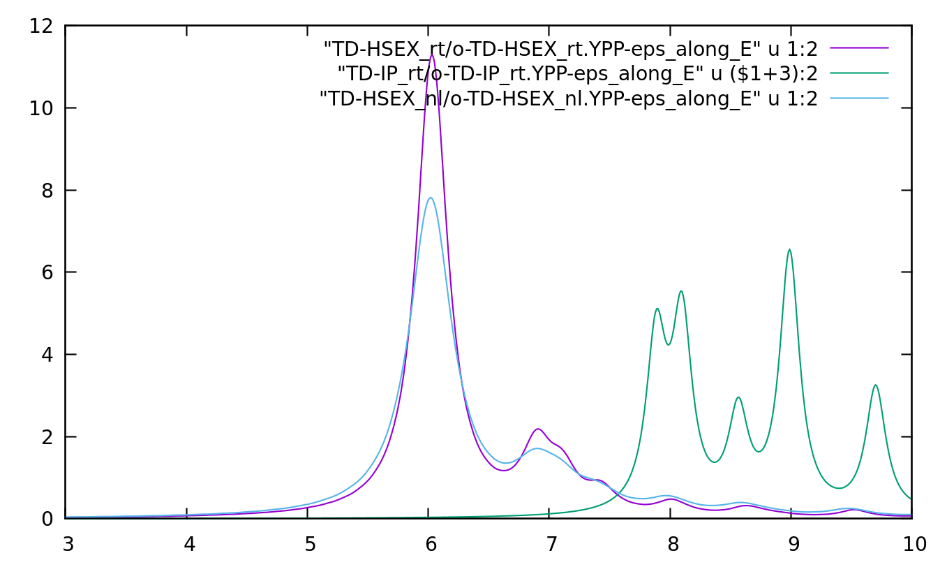
Plot the results:
gnuplot> set xrange [3:10]
gnuplot> set yrange [0:12]
gnuplot> plot "TD-SEX_nl/o-TD-SEX_nl.YPP-eps_along_E" u 1:2 w l
For comparison, the linear response results at the BSE level can be obtained following the BSE tutorial.
References
- ↑ I. Souza, J. Íñiguez, and D. Vanderbilt, PRB 69, 085106 (2004)
- ↑ 2.0 2.1 C. Attaccalite and M. Gruning Rev. B, 88, 235113 (2013)
- ↑ C. Attaccalite, arXiv 1609.09639 (2017)
- ↑ D. Sangalli, and A. Marini EPL 110, 47004 (2015)
- ↑ G. Strinati, La Rivista del Nuovo Cimento 11 (12), 1-86 (1988)
- ↑ C. Attaccalite, M. Grüning, and A. Marini PRB 84, 245110 (2011)
- ↑ Cite error: Invalid
<ref>tag; no text was provided for refs namedprb88


