Sum frequency generation

This tutorial is for internal use only, these response functions are not implemented/tested in yambo/yambopy suite.

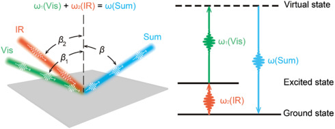
In this tutorial we will show you how to calculate Sum Frequency Generation(SFG) and also Difference Frequency Generation (DFG) in bulk materials.
We assume you are already familiar with the non-linear response using the Yambo code. If it is not the case please refer to the previous tutorials:
Linear response using Dynamical Berry Phase and Real time approach to non-linear response (SHG) and Ref..

This tutorial has been made possible thanks to the work of Mike N. Pionteck published in Ref. , results are also presented in this Libreoffice presentation and used for the tutorials on second/third harmonic generation: Real time approach to non-linear response (SHG). These new subroutine are available in the new YamboPy package. Hereafter the python script for the analysis:

from yambopy import *
from yambopy.nl.sum_frequencies import SF_Harmonic_Analysis
from yambopy.units import fs2aut
X_order=4
NLDB=YamboNLDB()
SF_Harmonic_Analysis(NLDB,X_order=X_order,T_range=[50.0*fs2aut,-1.0],prn_Peff=True,prn_Xhi=True)

Notice that we set the beginning of time range where analysis is performed with the variable T_range=[50.0*fs2aut,-1.0], you can also omit this variable and the code automatically will set the optimal range for the analysis using the damping given in input in the real-time simulation.
This script will analyse the real-time response and produce all the different [math]\displaystyle{ \chi^{(n)}(\omega) }[/math] in the form:

o.YamboPy-SF_probe_order_1_0 ==> [math]\displaystyle{ \chi^{(1)}(\omega=\omega_1) }[/math]
o.YamboPy-SF_probe_order_1_1 ==> [math]\displaystyle{ \chi^{(2)}(\omega=\omega_1+\omega_2) }[/math]
o.YamboPy-SF_probe_order_2_0 ==> [math]\displaystyle{ \chi^{(2)}(\omega=2\omega_1) }[/math]
o.YamboPy-SF_probe_order_0_2 ==> [math]\displaystyle{ \chi^{(2)}(\omega=2\omega_2) }[/math]
o.YamboPy-SF_probe_order_1_2 ==> [math]\displaystyle{ \chi^{(3)}(\omega=\omega_1+2\omega_2) }[/math]
o.YamboPy-SF_probe_order_2_2 ==> [math]\displaystyle{ \chi^{(4)}(\omega=2\omega_1+2\omega_2) }[/math]
etc....

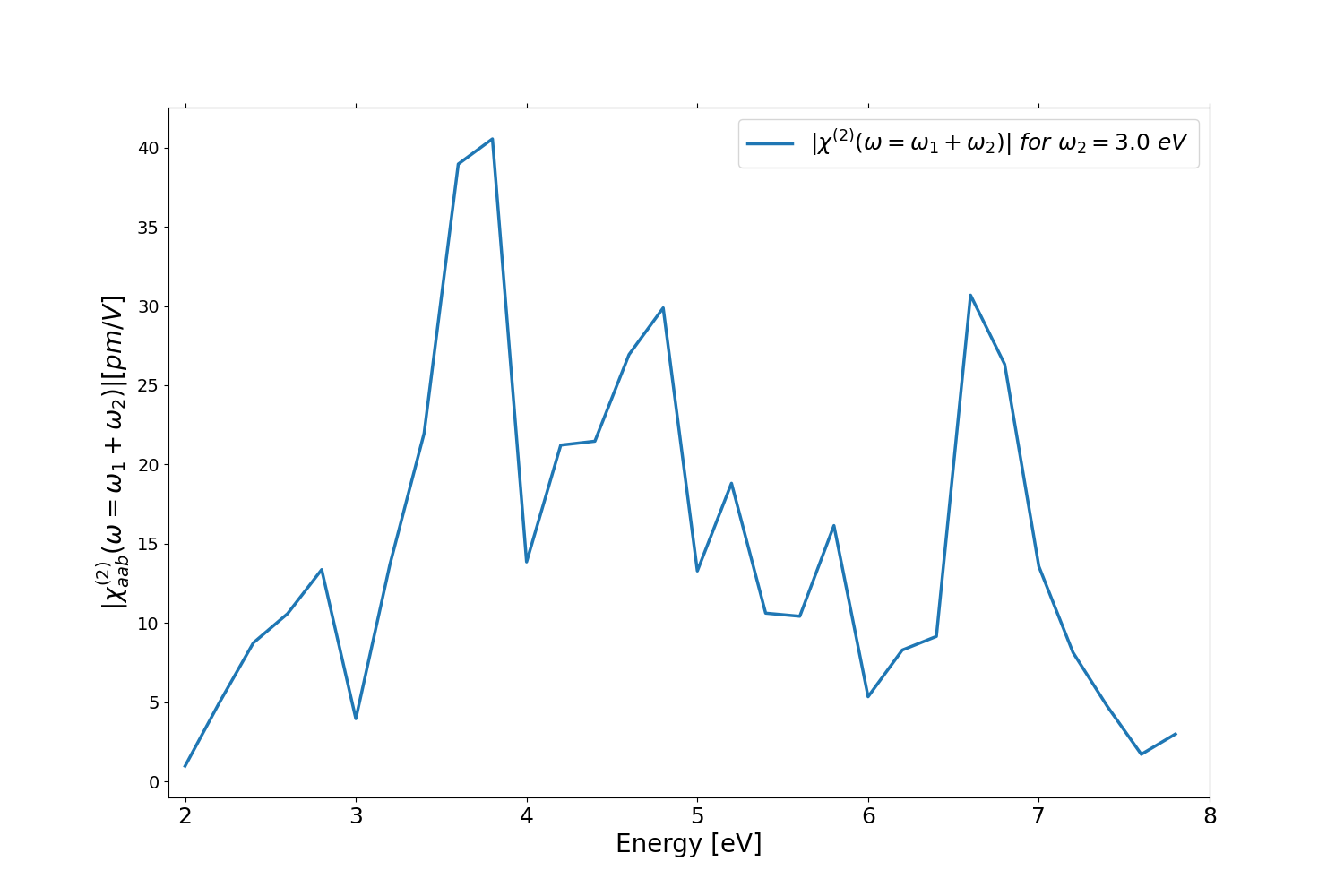
for example we can plot the 2 and 3 columns of the file o.YamboPy-SF_probe_order_1_1 that corresponds to the [math]\displaystyle{ \chi^{(2)}_{xyy} (\omega=\omega_1+\omega_2) }[/math] for [math]\displaystyle{ \omega_2 =3.0~eV }[/math]:

Here the python script used to generate the previous figure: plot_xhi2_monolayer.py

Checking the Fourier analysis

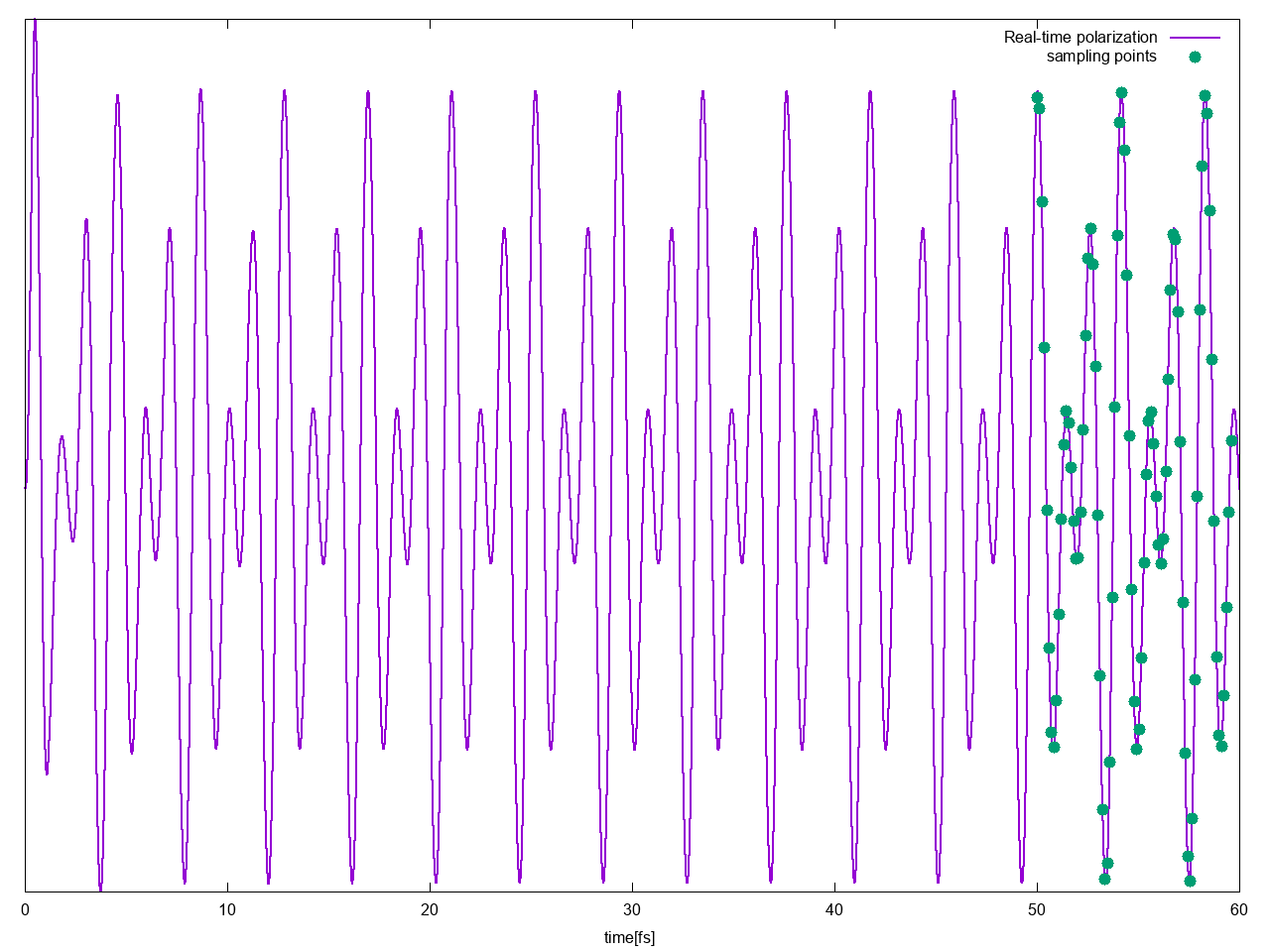
In the previous script we turned on the flag prn_Peff=True that automatically will produce a series of file to check if the Fourier was successful. The files o.YamboPy-sampling_F1 contain the sampling points used to fix the real-time polarization, you can for example plot o.YamboPy-sampling_F1 vs o.polarization_F1 together to see which part of [math]\displaystyle{ P(t) }[/math] is used to extract the response functions:

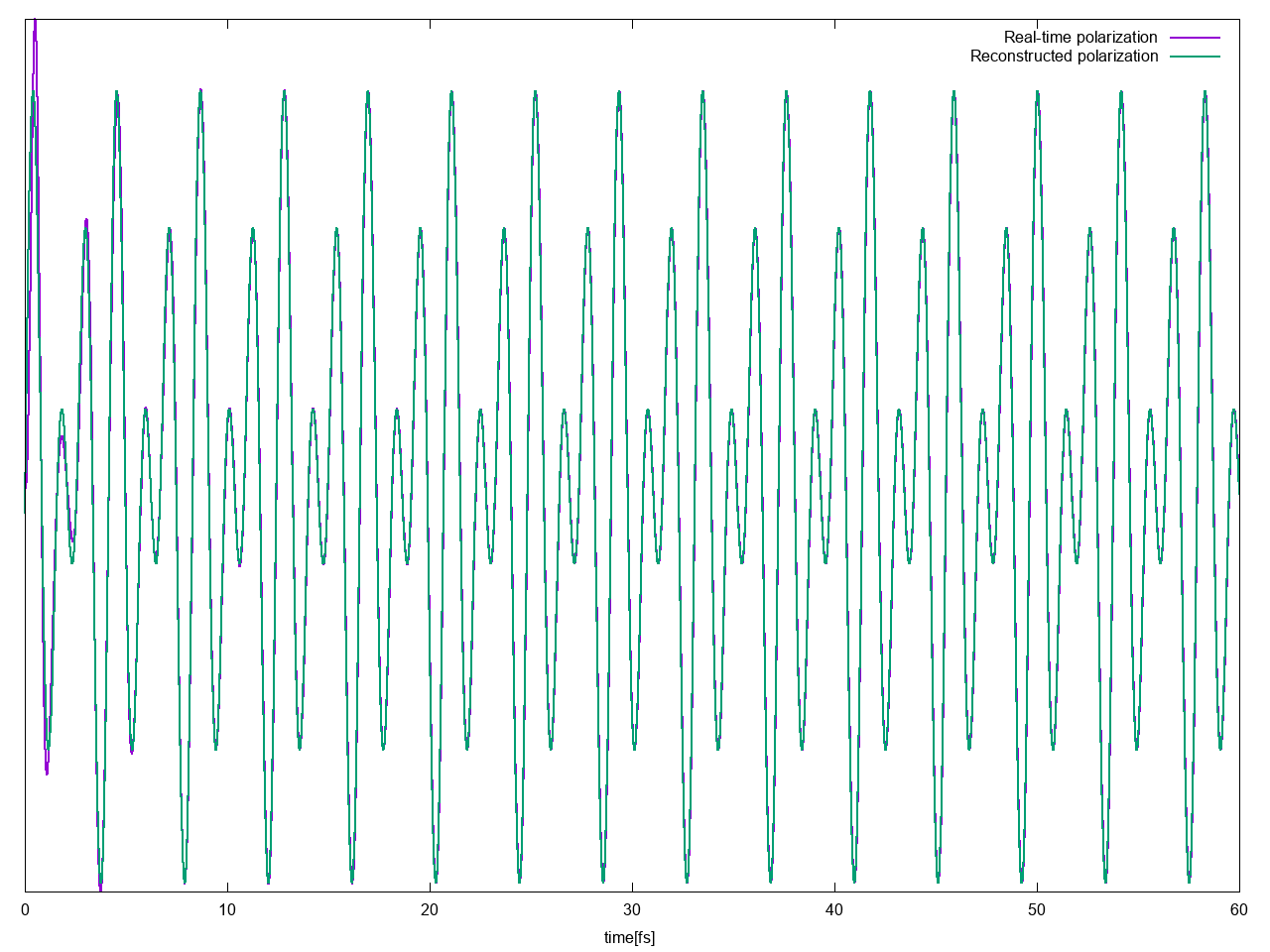
Then you can check if real-time polarization is well reconstructed by the Fourier coefficients calculated by the script by plotting o.YamboPy-pol_reconstructed_F1 vs o.polarization_F1

As you see the polarization is well reconstructed starting from the extracted Fourier coefficients, expect for the beginning, but this is normal because the initial signal is affected by the internal eigen--modes of the systems that later are washed out by the de-phasing. For this reason we use only the last part of the signal for the analysis, for more details see Ref.

Analysis of all runs

For this reason we provide you a simple python script to change also the frequency of the second field (in blue in the input).

run_many_sfg.py

please modify the python script by set the correct path of your executable, the parallelization and the number of frequency steps you are interested in. In this example we will do 30 frequency steps for both the first (in the Yambo input) and the second field (in the python script).

Calculations will take some time, in the above example we parallelized on 10 cores to speed up them.
When the calculations are terminated you will find many folders called EF1, EF2, ... EF29. These folders are generated from the loop on the second field frequency(Field2_Freq), and each one contains the response real-time polarization at 30 different frequencies of the first external field (Field1_Freq).

Now we will use a script to read all the real-time polarization, Fourier analyze them as it was done in the previous section for a single one, and the write the [math]\displaystyle{ \chi^{(2)}(\omega=\omega_1 + \omega_2) }[/math] in a file in the form: [math]\displaystyle{ \omega_1 , \omega_2, Re \{\chi^{(2)}\} , Im \{\chi^{(2)}\} }[/math].

analysis_sfg.py

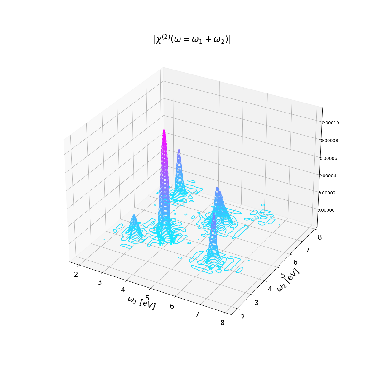
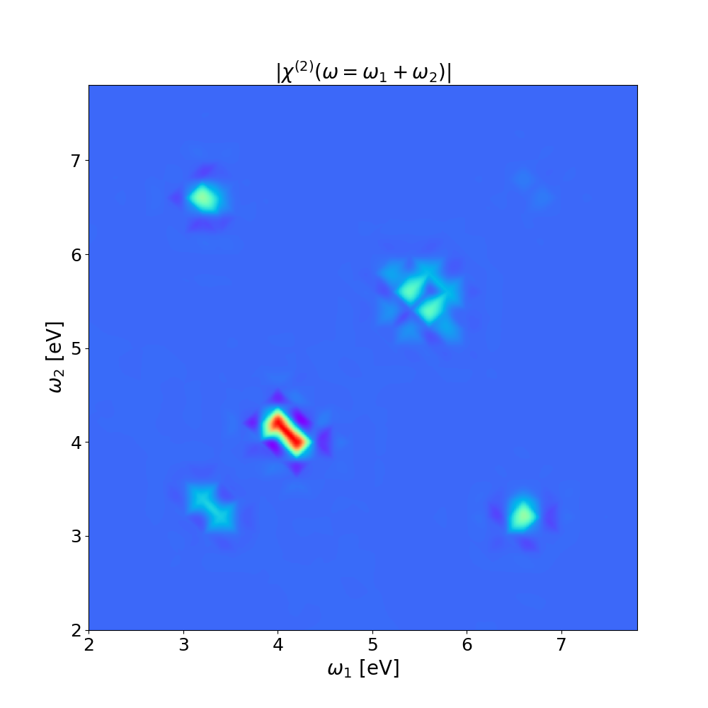
then we can interpolate the results [math]\displaystyle{ \chi^{(2)}(\omega) }[/math] and plot results in 3D or 2D: plot_xhi_2d.py, plot_xhi_3d.py

You can compare these results with those of Ref.. Note that in order to get fully converged results, you need to increase: the number of k-points, the length of the simulations, and the number of frequencies used in the plots. Converged parameters for this system can be found in Ref., including all details to include excitonic effects.
Important: In case of degenerate or multiple frequencies [math]\displaystyle{ \omega_1 = n \omega_2 }[/math] where [math]\displaystyle{ n }[/math] is an integer, the algorithm used to extract the SFG/DFG coefficient could not converge. In this case you can discard these points and use the neighbour solution for interpolation, see discussion in reference . Another possibility is to use a least-squares fit algohrithm that starts from the neighbour solution to find the SFG/DFG coefficents, this is implemented in YamboPy in the sum_frequency.py file, but is commented.

Comparison with SHG

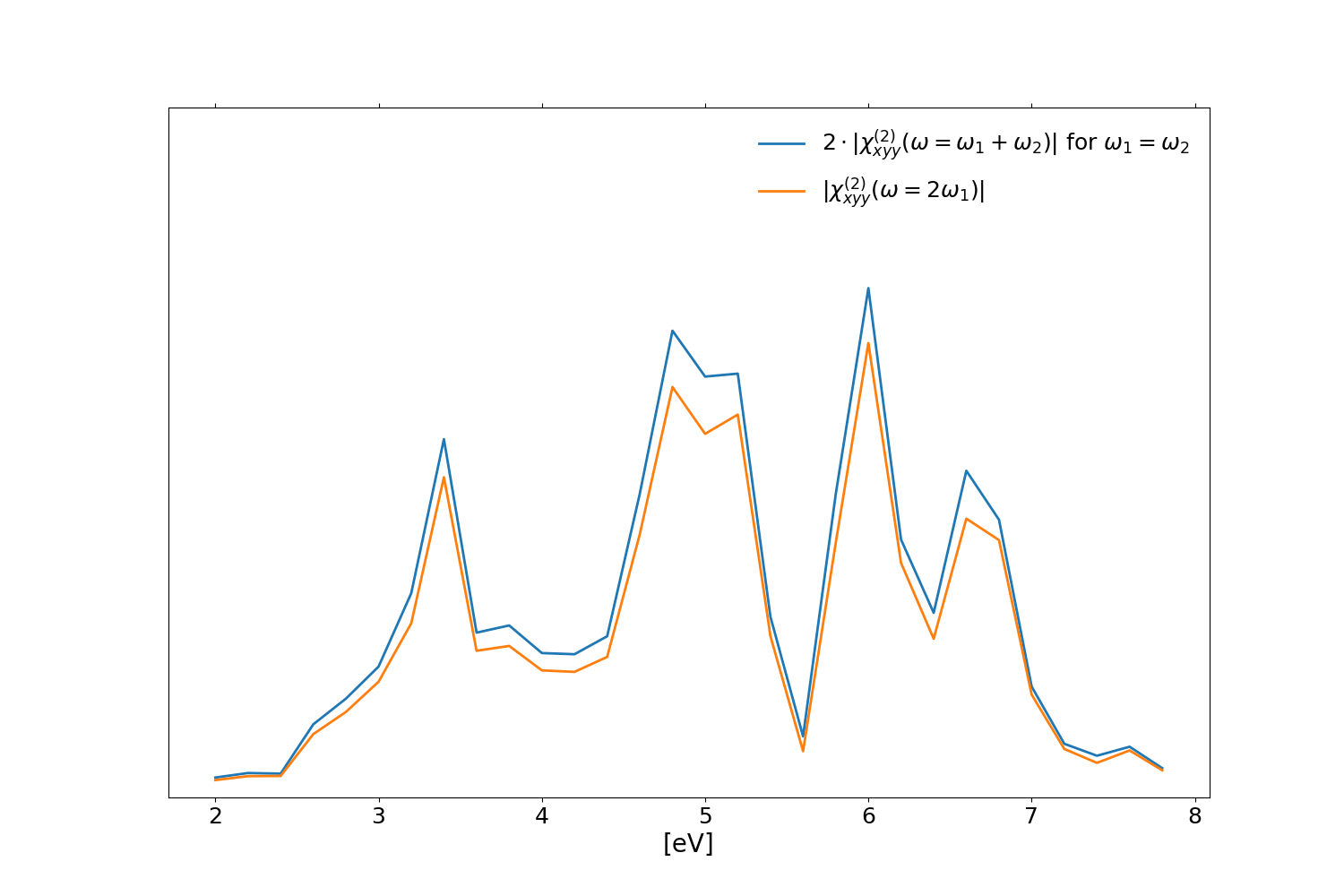
Finally you can compare the diagonal of [math]\displaystyle{ \chi^{(2)}(\omega=\omega_1 +\omega_2) }[/math], when [math]\displaystyle{ \omega_1 =\omega_2 }[/math], with the standard second harmonic generation [math]\displaystyle{ \chi^{(2)}(\omega=2 \omega_1) }[/math] calculated as explained in the tutorial Real time approach to non-linear response (SHG):

Notice that there is factor two between the two response functions, this is the so-called degeneracy factor, for more details see Sec. 1.3 in Ref.. The small differences between the two spectra are given the different sampling strategies of the SF_Harmonic_Analysis function respect to the Harmonic_Analysis one.