Two-photon absorption
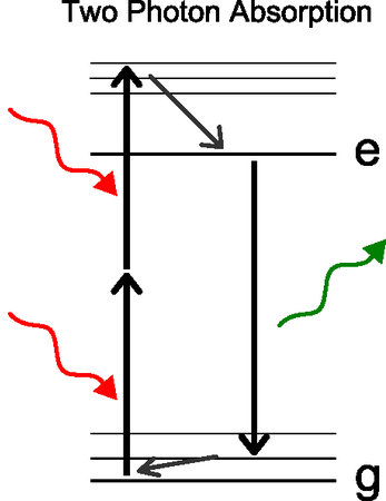
In this tutorial we will show how to calculate two-photon absorption(TPA) in bulk silicon, following the approach descried in Ref. [1].
In this tutorial we suppose you are already familiar with the non-linear response using the Yambo code.
If it is not the case please study the previous tutorials: Linear response using Dynamical Berry Phase and Real time approach to non-linear response (SHG).
The tutorial is divided in different steps from the DFT calculation to the final TPA spectrum. For the calculation of the TPA we will use the real-time approach proposed in Ref. [2]
DFT calculations
Here we provide input files for QuantumEspresso both the self-consistent calculation and the non-self-consistent: QE_silicon.tgz
Run them, import the wave-function in Yambo and run the setup. (see previous tutorials).
Removing symmetries
In this tutorial we will calculate the TPA along the 'x' direction therefore we remove symmetries not compatible with an external field along this direction, with the command ypp_nl -y:
fixsyms                          # [R] Remove symmetries not consistent with an
external perturbation
% Efield1
  1.000000 | 0.000000 | 0.000000 |        # First external Electric Field
%
% Efield2
 0.000000 | 0.000000 | 0.000000 |        # Additional external Electric Field
%
BField= 0.000000           T     # [MAG] Magnetic field modulus
Bpsi= 0.000000             deg   # [MAG] Magnetic field psi angle [degree]
Btheta= 0.000000           deg   # [MAG] Magnetic field theta angle [degree]
#RmAllSymm                     # Remove all symmetries
RmTimeRev                     # Remove Time Reversal
#RmSpaceInv                    # Remove Spatial Inversion
the you can go in the FixSymm folder and run the setup again.
Calculations at different field intensities
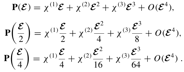
In order to extract the TPA coefficient we will run a series of simulation at different intensities of the external field: Ε, Ε/2, Ε/4. The polarization obtained from these simulation can be expanded in the field as:
then we will combine them to obtain the TPA coefficient as:
for more detail see Ref.[1]. Hereafter the inputs for the real-time simulation. These inputs can be generated using the command yambo -u n -V qp. The first input that we will callinput1.in reads:
nloptics                         # [R] Non-linear spectroscopy
% NLBands
   1 | 7 |                           # [NL] Bands range
%
NLverbosity= "low"               # [NL] Verbosity level (low | high)
NLtime=74.000000           fs    # [NL] Simulation Time
NLstep= 0.002500           fs    # [NL] Time step length
NLintegrator= "INVINT"           # [NL] Integrator ("EULEREXP/RK2/RK4/RK2EXP/HEUN/INVINT/CRANKNIC")
NLCorrelation= "IPA"             # [NL] Correlation ("IPA/HARTREE/TDDFT/LRC/LRW/JGM/SEX")
NLLrcAlpha= 0.000000             # [NL] Long Range Correction
% NLEnRange
  0.200000 | 5.000000 |         eV    # [NL] Energy range
%
NLEnSteps= 24                   # [NL] Energy steps
NLDamping= 0.100000        eV    # [NL] Damping (or dephasing)
#EvalCurrent                   # [NL] Evaluate the current
% Field1_Dir
   1.000000 | 0.000000 | 0.000000 |        # [NL Field1] Field Versor
%
Field1_kind= "SIN"             # [NL Field1] Kind(SIN|SOFTSIN|RES|ANTIRES|GAUSS|DELTA|QSSIN)
% GfnQP_E
 0.600000 | 1.000000 | 1.000000 |        # [EXTQP G] E parameters  (c/v) eV|adim|adim
%
Field1_Int=4.0000E+4         kWLm2 # [NL Field1] Intensity
Field1_Tstart= 0.000000      fs    # [NL Field1] Initial Time
the second and third input files (input2.in and input3.in) are equivalent to the first one but with different field intensities: Field1_Int=1.0000E+4 and Field1_Int=0.2500E+4/
Then you can run the three simulations with the command:
yambo -J input1.in -J RUN1
yambo -J input2.in -J RUN2
yambo -J input3.in -J RUN3
Nota bene: these runs are long, they will take approximativelly 3 hours on a serial machine. In order to speed up them you can decrease NLEnSteps=12
or you can run in parallel and add two lines at the beginning of the input:
NL_CPU= "12 1"                    # [PARALLEL] CPUs for each role
NL_ROLEs= "w k"                  # [PARALLEL] CPUs roles (w,k)
where 12 is the number of core you want to use. The best is to use a divisor of 24 (number of energy steps).
Perform Fourier analysis of the polarization
When real-time simulation are terminated, we can use ypp_nl to analyze the real-time polarization
in a way similar to the tutorial on second harmonic generation (Real time approach to non-linear response (SHG)).
The ypp_fourier.in input, generated with the commanda ypp_nl -u, reads:
nonlinear                        # [R] Non-linear response analysis
Xorder= 5                        # Max order of the response/exc functions
% TimeRange
-1.000000 |-1.000000 |         fs    # Time-window where processing is done
# From here onwards, it is ignored in SHG
%
ETStpsRt= 200                    # Total Energy steps
% EnRngeRt
  0.00000 | 10.00000 |         eV    # Energy range
%
DampMode= "NONE"                 # Damping type ( NONE | LORENTZIAN | GAUSSIAN )
DampFactor= 0.000000       eV    # Damping parameter
you can do:
ypp_nl -F ypp_fourier.in -J RUN1
ypp_nl -F ypp_fourier.in -J RUN2
ypp_nl -F ypp_fourier.in -J RUN3
this will produce the corresponding coefficients χ1(ω)=P(ω)/E(ω), χ2(2ω)=P(2ω)/E2(ω), χ3, etc.. in the file o-RUN1.YPP-order ...
Use Richardson extrapolation to extract the TPA
Finally we will use the formula:
to combine the different polarization and extract the TPA coefficient. This can be done using the following script: [[1]]
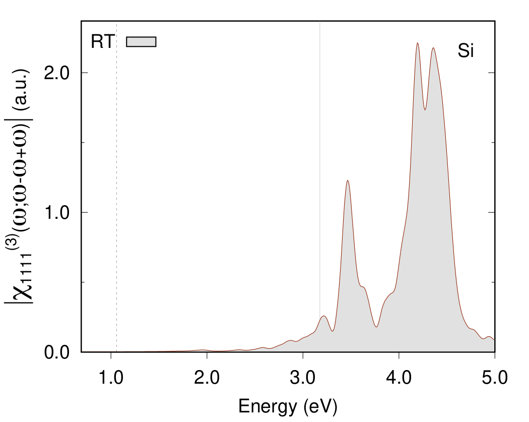
This result was calculated with few energy steps (NLEnSteps= 24) but if you increase this number you can get a smooth result. For example in the figure below we used 481 points.
References
- ↑ 1.0 1.1 Two-photon absorption in two-dimensional materials: The case of hexagonal boron nitride Claudio Attaccalite, Myrta Grüning, Hakim Amara, Sylvain Latil, and François Ducastelle Phys. Rev. B 98, 165126 (2018)
- ↑ Nonlinear optics from an ab initio approach by means of the dynamical Berry phase: Application to second- and third-harmonic generation in semiconductors, C. Attaccalite and M. Grüning, Phys. Rev. B 88, 235113(2013)


