Pump and Probe
In this tutorial we will show you how to setup two external fields in yambo_nl, to perform pump and probe simulation. [1]
This tutorial is at independent particle level, but the same kind of simulation can be repeated including local field effects,
quasi-particle correction or electron-hole interaction, see for example the tutorials:
Correlation effects in the non-linear response
Real time Bethe-Salpeter Equation (TDSE)
This tutorial supposes that you are already familiar with real-time simulation with Yambo[2]
if it is not the case please check these tutorials: Tutorials#Non_linear_response
We start from the h-BN monolayer with an in place lattice constant a=2.5 Å and a box large 33 a.u. in the z-direction.
Standard DFT input for hBN monolayer for ABINIT or QuantumEspresso can be found here Tutorials.
We used a 9x9x1 k-points grid and 8 bands in the non-self consistent calculation and 40 Ry cutoff for the wave-function.
In our example we choose direction [0,1,0] for the pump and [1,0,0] for the probe. We generate the ypp.in to remove symmetries with the command ypp -y and we modify it as:
fixsyms                          # [R] Remove symmetries not consistent with an external perturbation
% Efield1
 0.000000 | 1.000000 | 0.000000 |        # First external Electric Field
%
% Efield2
 1.000000 | 0.000000 | 0.000000 |        # Additional external Electric Field
%
BField= 0.000000           T     # [MAG] Magnetic field modulus
Bpsi= 0.000000             deg   # [MAG] Magnetic field psi angle [degree]
Btheta= 0.000000           deg   # [MAG] Magnetic field theta angle [degree]
#RmAllSymm                     # Remove all symmetries
RmTimeRev                     # Remove Time Reversal
#RmSpaceInv                    # Remove Spatial Inversion
then we go in the FixSymm directory and run again the setup.
We will perform three different real-time calculations:
- the probe field alone;
- the pump field alone;
- the pump and probe configuration.
Probe only
We can generate the input file for a generic Pump and Probe calculations with the command: yambo_nl -u p -F yambo.in_probe:
nloptics                         # [R] Non-linear spectroscopy
DIP_Threads=0                    # [OPENMP/X] Number of threads for dipoles
NL_Threads=0                     # [OPENMP/NL] Number of threads for nl-optics
% NLBands
    3 |  6 |                           # [NL] Bands range
%
NLverbosity= "high"              # [NL] Verbosity level (low | high)
NLtime=  80.000000           fs    # [NL] Simulation Time
NLintegrator= "  CRANKNIC"           # [NL] Integrator ("EULEREXP/RK2/RK4/RK2EXP/HEUN/INVINT/CRANKNIC")
NLCorrelation= "IPA"             # [NL] Correlation ("IPA/HARTREE/TDDFT/LRC/LRW/JGM/SEX")
NLLrcAlpha= 0.000000             # [NL] Long Range Correction
NLDamping= 0.000000        eV    # [NL] Damping (or dephasing)
RADLifeTime=-1.000000      fs    # [RT] Radiative life-time (if negative Yambo sets it equal to Phase_LifeTime in NL)
#EvalCurrent                   # [NL] Evaluate the current
#FrPolPerdic                   # [DIP] Force periodicity of polarization respect to the external field
HARRLvcs= 21817            RL    # [HA] Hartree     RL components
EXXRLvcs= 21817            RL    # [XX] Exchange    RL components
% Field1_Freq
 0.100000 | 0.100000 |         eV    # [RT Field1] Frequency
%
Field1_NFreqs= 1                 # [RT Field1] Frequency
Field1_Int=  1000.00       kWLm2 # [RT Field1] Intensity
Field1_Width= 0.000000     fs    # [RT Field1] Width
Field1_kind= "  DELTA"           # [RT Field1] Kind(SIN|COS|RES|ANTIRES|GAUSS|DELTA|QSSIN)
Field1_pol= "linear"             # [RT Field1] Pol(linear|circular)
% Field1_Dir
   0.000000 | 1.000000 | 0.000000 |        # [RT Field1] Versor
%
Field1_Tstart=   5.00000    fs    # [RT Field1] Initial Time
[......]
In this input we set only the first field that is the probe, we use a DELTA function as field in such a way to probe all the frequencies, and set the starting point of the delta at t=5 fs.
Run this job in a separate folder with the command yambo_nl -F yambo.in_probe -J PROBE. Then we can analyze the spectra with ypp -u -J PROBE :
nonlinear                        # [R] Non-linear response analysis
Xorder= 1                        # Max order of the response/exc functions
% TimeRange
-1.000000 |-1.000000 |         fs    # Time-window where processing is done
%
ETStpsRt= 200                    # Total Energy steps
% EnRngeRt
  0.00000 | 20.00000 |         eV    # Energy range
%
DampMode= "LORENTZIAN"           # Damping type ( NONE | LORENTZIAN | GAUSSIAN )
DampFactor= 0.100000       eV    # Damping parameter
PumpPATH= "none"           # Path of the simulation with the Pump only
and get the dielectric response. Notice that we introduce a Lorentzian broadening the post-processing.
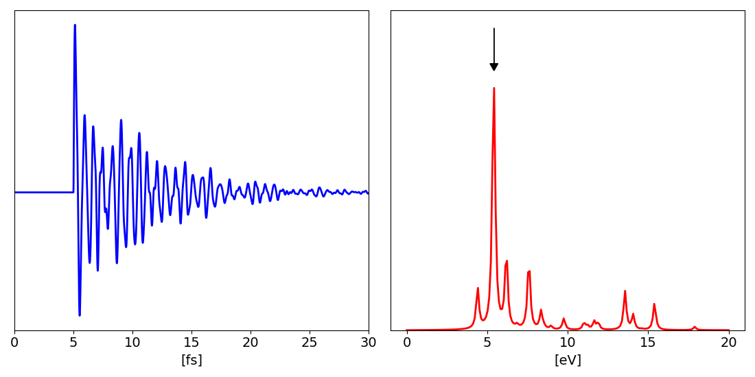
Hereafter we plot the damped polarization along the y-direction and the corresponding dielectric constant:
the arrow indicates the position where we will put the Pump in the next simulation.
Pump only
Now we run a simulation with the pump field only. We generate the input in the same way yambo_nl -u p -F yambo.in_pump.
These result will be our reference field in the final analysis. Here the input file for the pump:
nloptics                         # [R] Non-linear spectroscopy
DIP_Threads=0                    # [OPENMP/X] Number of threads for dipoles
NL_Threads=0                     # [OPENMP/NL] Number of threads for nl-optics
% NLBands
   3 |  6 |                           # [NL] Bands range
%
NLverbosity= "high"              # [NL] Verbosity level (low | high)
NLtime=  150.0000           fs    # [NL] Simulation Time
NLintegrator= "CRANKNIC"         # [NL] Integrator ("EULEREXP/RK2/RK4/RK2EXP/HEUN/INVINT/CRANKNIC")
NLCorrelation= "IPA"             # [NL] Correlation ("IPA/HARTREE/TDDFT/LRC/LRW/JGM/SEX")
NLLrcAlpha= 0.000000             # [NL] Long Range Correction
NLDamping= 0.000000        eV    # [NL] Damping (or dephasing)
RADLifeTime=-1.000000      fs    # [RT] Radiative life-time (if negative Yambo sets it equal to Phase_LifeTime in NL)
#EvalCurrent                   # [NL] Evaluate the current
#FrPolPerdic                   # [DIP] Force periodicity of polarization respect to the external field
HARRLvcs= 21817            RL    # [HA] Hartree     RL components
EXXRLvcs= 21817            RL    # [XX] Exchange    RL components
% Field1_Freq
 0.100000 | 0.100000 |         eV    # [RT Field1] Frequency
%
Field1_NFreqs= 1                 # [RT Field1] Frequency
Field1_Int=  10000.00       kWLm2 # [RT Field1] Intensity
Field1_Width= 0.000000     fs    # [RT Field1] Width
Field1_kind= "SOFTSIN"           # [RT Field1] Kind(SIN|COS|RES|ANTIRES|GAUSS|DELTA|QSSIN)
Field1_pol= "linear"             # [RT Field1] Pol(linear|circular)
% Field1_Dir
 0.000000 | 0.000000 | 0.000000 |        # [RT Field1] Versor
%
Field1_Tstart= 0.010000    fs    # [RT Field1] Initial Time
% Field2_Freq
  5.42 | 5.42 |         eV    # [RT Field2] Frequency
%
Field2_NFreqs= 1                 # [RT Field2] Frequency
Field2_Int=  1000.00       kWLm2 # [RT Field2] Intensity
Field2_Width= 10.00000     fs    # [RT Field2] Width
Field2_kind= "QSSIN"             # [RT Field2] Kind(SIN|COS|RES|ANTIRES|GAUSS|DELTA|QSSIN)
Field2_pol= "linear"             # [RT Field2] Pol(linear|circular)
% Field2_Dir
 0.000000 | 1.000000 | 0.000000 |        # [RT Field2] Versor
%
Field2_Tstart= 0.010000    fs    # [RT Field2] Initial Time
[...]
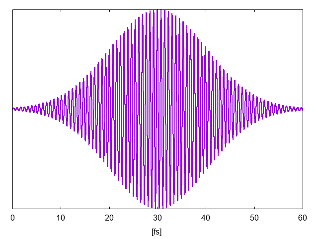
In this simulation we used as Pump field QSSIN that is sinus with a Guassian envelopesine-Gaussian wave. For a list of all possible field in Yambo see the file src/modules/mod_fields.F. We centred the field frequency at 5.22 eV that is the energy of the highest peak in the previous figure, see arrow there. Run the simulation with the command yambo_nl -F yambo.in_pump -J PUMP . The pump field (column 6th of the file o-PUMP.external_potential_F1) is shown in the figure below:
Pump and probe
Now we copy the pump in file in a new file cp yambo.in_pump yambo.in_pump_and_probe and turn on the probe field:
nloptics                         # [R] Non-linear spectroscopy
DIP_Threads=0                    # [OPENMP/X] Number of threads for dipoles
NL_Threads=0                     # [OPENMP/NL] Number of threads for nl-optics
% NLBands
  3 |  6 |                           # [NL] Bands range
%
NLverbosity= "high"              # [NL] Verbosity level (low | high)
NLtime=  150.0000           fs    # [NL] Simulation Time
NLintegrator= "CRANKNIC"         # [NL] Integrator ("EULEREXP/RK2/RK4/RK2EXP/HEUN/INVINT/CRANKNIC")
NLCorrelation= "IPA"             # [NL] Correlation ("IPA/HARTREE/TDDFT/LRC/LRW/JGM/SEX")
NLLrcAlpha= 0.000000             # [NL] Long Range Correction
NLDamping= 0.000000        eV    # [NL] Damping (or dephasing)
RADLifeTime=-1.000000      fs    # [RT] Radiative life-time (if negative Yambo sets it equal to Phase_LifeTime in NL)
#EvalCurrent                   # [NL] Evaluate the current
#FrPolPerdic                   # [DIP] Force periodicity of polarization respect to the external field
HARRLvcs= 21817            RL    # [HA] Hartree     RL components
EXXRLvcs= 21817            RL    # [XX] Exchange    RL components
% Field1_Freq
 0.100000 | 0.100000 |         eV    # [RT Field1] Frequency
%
Field1_NFreqs= 1                 # [RT Field1] Frequency
Field1_Int=  1.00       kWLm2 # [RT Field1] Intensity
Field1_Width= 0.000000     fs    # [RT Field1] Width
Field1_kind= "DELTA"           # [RT Field1] Kind(SIN|COS|RES|ANTIRES|GAUSS|DELTA|QSSIN)
Field1_pol= "linear"             # [RT Field1] Pol(linear|circular)
% Field1_Dir
 1.000000 | 0.000000 | 0.000000 |        # [RT Field1] Versor
%
Field1_Tstart= 90.0000    fs    # [RT Field1] Initial Time
% Field2_Freq
  5.42 | 5.42 |         eV    # [RT Field2] Frequency
%
Field2_NFreqs= 1                 # [RT Field2] Frequency
Field2_Int=  1000.00       kWLm2 # [RT Field2] Intensity
Field2_Width= 10.00000     fs    # [RT Field2] Width
Field2_kind= "QSSIN"             # [RT Field2] Kind(SIN|COS|RES|ANTIRES|GAUSS|DELTA|QSSIN)
Field2_pol= "linear"             # [RT Field2] Pol(linear|circular)
% Field2_Dir
 0.000000 | 1.000000 | 0.000000 |        # [RT Field2] Versor
%
Field2_Tstart= 0.010000    fs    # [RT Field2] Initial Time
you run the simulation with the command yambo_nl -F yambo.in_pump_and_probe -J PUMP_AND_PROBE and then we analyze the result using ypp with the command: ypp_nl -u -J PUMP_AND_PROBE :
nonlinear                        # [R] Non-linear response analysis
Xorder= 1                        # Max order of the response/exc functions
% TimeRange
-1.000000 |-1.000000 |         fs    # Time-window where processing is done
%
ETStpsRt= 500                    # Total Energy steps
% EnRngeRt
  0.00000 | 3.9000 |         eV    # Energy range
%
DampMode= "GAUSSIAN"                 # Damping type ( NONE | LORENTZIAN | GAUSSIAN )
DampFactor= 0.085000       eV    # Damping parameter
PumpPATH= "./PUMP/"                 # Path of the simulation with the Pump only
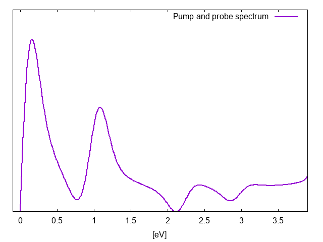
Notice that in this case we are interested in the spectra below the 4 eV, that is was zero without the presence of the pump. We put in the input the pump path in such way to calculate polarization of the pump&probe minus the one of generate by the pump only [math]\displaystyle{ \Delta P(t) = P_{PnP}(t) - P_{pump}(t) }[/math]. Then we analyze the [math]\displaystyle{ \Delta P(t) }[/math] and get the new spectra:
The peak that you see in this spectrum, that were not present in when the pump was zero, correspond to the transition between the different excited states. The pump field populates the state at 5.42 eV and then the probe excites electrons from this state to higher states. The energy difference between the higher excited states and the peak at 5.42 define the position of the peaks in the pump and probe spectrum, while their intensity is dictated by the dipole matrix elements between the different excited states, see Ref. [1].
Additional comments on pump and probe calculations
- We used a Gaussian damping factor, this choice is motivated by various tests we have done, and it seems to us that in pump and probe this broadening gives better results.
- If you plot all spectrum you will notice that the "equilibrium part" is much stronger than the one induced by the pump, this is normal because only a small fraction of electron are promoted in the excited state by the pump.
- All previous simulation can be run also in presence of excitons, see Ref. [1] and group theory can be used to predict dark/bright transition in the pump and probe spectroscopy.[3]
- In principle is it possible to include damping and radiative life-time in the simulation to study retardation effect between the pump and probe. This approach exact in the independent particle case, but introduces an error when correlation effects are present, see Refs.[4] and [5]for a discussion.
- Non-linear response (SHG, THG, ...) induced by the pump is not implemented yet... if you have a good idea how to do it, please let us know
Analysis of the results using YamboPy
This part works only with Yambo 5.3 or the last version available on Github: https://github.com/yambo-code/yambo
References
- ↑ 1.0 1.1 1.2 Exciton - Exciton transitions involving strongly bound excitons: an ab-initio approach, D. Sangalli, M. D'Alessandro and C. Attaccalite, Physical Review B 107 (20), 205203 (2023)
- ↑ Non-linear response in extended systems: a real-time approach, C. Attaccalite
- ↑ Group Theory, Application to the Physics of Condensed Matter, Mildred S. S. Dresselhaus, Gene Dresselhaus, Ado Jorio, Springer Editor
- ↑ Excitons and carriers in transient absorption and time-resolved ARPES spectroscopy: an abinitio approach, D. Sangalli, Phys. Rev. Materials 5, 083803 (2021)
- ↑ Theory of exciton-phonon coupling, Gabriel Antonius and Steven G. Louie Phys. Rev. B 105, 085111 (2022)


