Quasi-particles of a 2D system
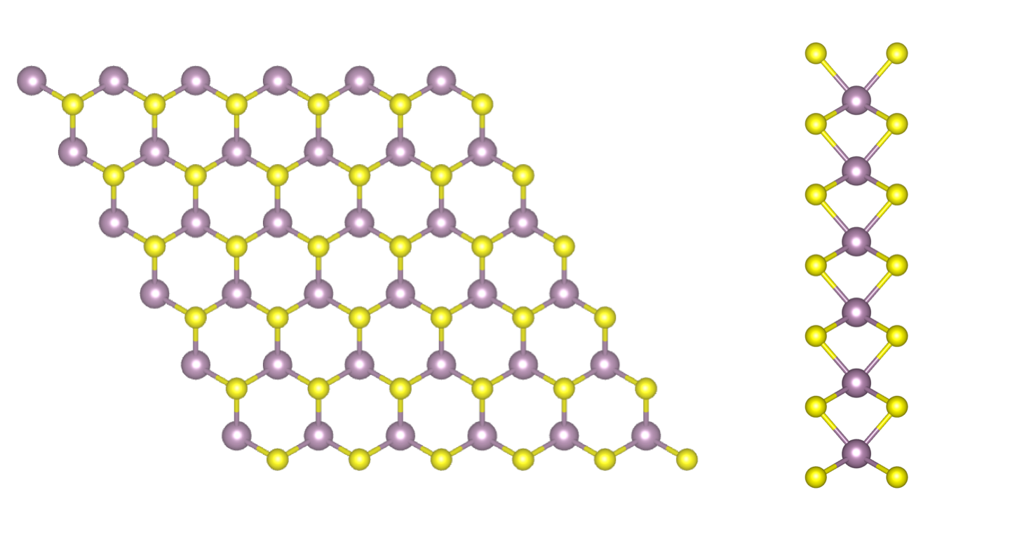
In this tutorial you will compute the quasiparticle corrections to the band structure of a free-standing single layer of MoS2. Aim of the tutorial is to learn how to efficiently run a GW simulation in a 2D material based on:
- Acceleration techniques of GW, some of which specific for 2D systems
- Parallelization techniques
In the end, you will obtain a quasiparticle band structure based on the simulations, the first step towards the reproduction of an ARPES spectrum. Beware: we won’t use fully converged parameters, so the final result should not be considered very accurate.
Step 1: Speeding up the self-energy convergence
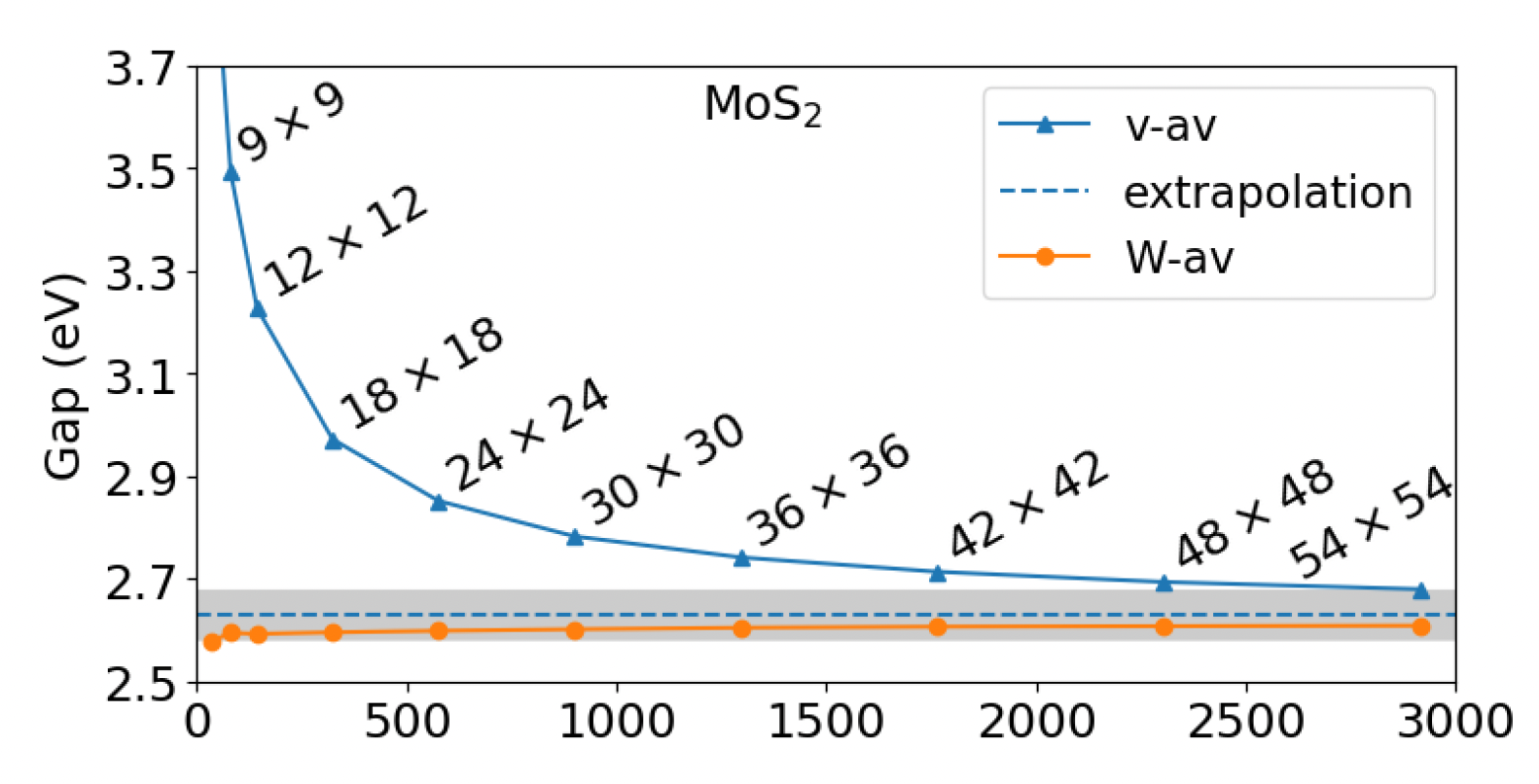
In this section, you will learn to use two algorithms present in Yambo that lead to a speed up of the self-energy convergence with respect to the k-grid.
To appreciate the impact of these algorithms, let us first perform a GW computation for the monolayer of MoS2. Enter the 01_GW_first_run folder
As in the GW basics tutorial, we generate an input file with:
yambo -F gw_ppa.in -p p
The input file reads:
gw0                              # [R] GW approximation
ppa                              # [R][Xp] Plasmon Pole Approximation for the Screened Interaction
dyson                            # [R] Dyson Equation solver
HF_and_locXC                     # [R] Hartree-Fock
em1d                             # [R][X] Dynamically Screened Interaction
X_Threads=0                      # [OPENMP/X] Number of threads for response functions
DIP_Threads=0                    # [OPENMP/X] Number of threads for dipoles
SE_Threads=0                     # [OPENMP/GW] Number of threads for self-energy
EXXRLvcs=  37965           RL    # [XX] Exchange    RL components
VXCRLvcs=  37965           RL    # [XC] XCpotential RL components
Chimod= "HARTREE"                # [X] IP/Hartree/ALDA/LRC/PF/BSfxc
% BndsRnXp
   1 | 80 |                       # [Xp] Polarization function bands
%
NGsBlkXp= 10                Ry    # [Xp] Response block size
% LongDrXp
1.000000 | 1.000000 | 1.000000 |        # [Xp] [cc] Electric Field
%
PPAPntXp= 27.21138         eV    # [Xp] PPA imaginary energy
XTermKind= "none"                # [X] X terminator ("none","BG" Bruneval-Gonze)
% GbndRnge
   1 | 80 |                         # [GW] G[W] bands range
%
GTermKind= "BG"                  # [GW] GW terminator ("none","BG" Bruneval-Gonze,"BRS" Berger-Reining-Sottile)
DysSolver= "n"                   # [GW] Dyson Equation solver ("n","s","g")
%QPkrange                        # [GW] QP generalized Kpoint/Band indices
7|7|13|14|
%
Here, consider the number of G vectors and the number of bands as already being converged. So, compute the gap at GW level:
yambo -F gw_ppa.in -J 80b_10Ry
Once terminated the computation, you can now inspect the output file o-80b_10Ry.qp.
You should have obtained a GW gap of 2.483 eV.
RIM
To understand how we can improve the calculation in the k-grid to achieve a speed-up, consider briefly again the expression of the exchange part of the self-energy
You can notice that the integration around q=0 here is problematic for the presence of a 1/q from the Coulomb potential that diverges, while all the other terms are slowly varying in q. Usually in Yambo this integration is performed analytically in a small sphere around q=0.
However, in this way the code lost part of the integral out of the circle. This usually
is not problematic because for a large number of q and k point the missing term goes to zero.
However in system that requires few k-points or even only the gamma one, it is possible
to perform a better integration of this term by adding the flag -r. So as
yambo -F gw_ppa.in -p p -r
In this manner, you generate the input:
HF_and_locXC                 # [R XX] Hartree-Fock Self-energy and Vxc
ppa                          # [R Xp] Plasmon Pole Approximation
gw0                          # [R GW] G0W0 Quasiparticle energy levels
em1d                         # [R Xd] Dynamical Inverse Dielectric Matrix
rim_cut                      # [R] Coulomb potential
RandQpts=  1000000           # [RIM] Number of random q-points in the BZ
RandGvec=  100           RL  # [RIM] Coulomb interaction RS components
CUTGeo= "slab z"             # [CUT] Coulomb Cutoff geometry: box/cylinder/sphere/ws/slab X/Y/Z/XY..
...
In this input, RandGvec is the number of component of the Coulomb potential we want integrate numerically and RandQpts is the number of random points used to perform the integral by Monte Carlo.
The [CUT] keyword refers to the truncation of the Coulomb interaction to avoid spurious interaction between periodically repeated copies of the simulation supercell along the z-direction (that in this case is the non periodic direction). Keep in mind that the vacuum space between two copies of the system should be converged: here we are using 20 bohr but a value of 40 bohr would be more realistic.
If you turn on this integration you will get a slightly different band gap, but in the limit of large k points the final results will be the same of the standard method. However this correction is important for systems that converge with few k-points or with gamma only and it is applied both at the exchange and correlation part of the self-energy.
Now make a GW computation using the RIM method
gw0                              # [R] GW approximation
ppa                              # [R][Xp] Plasmon Pole Approximation for the Screened Interaction
dyson                            # [R] Dyson Equation solver
HF_and_locXC                     # [R] Hartree-Fock
em1d                             # [R][X] Dynamically Screened Interaction
X_Threads=0                      # [OPENMP/X] Number of threads for response functions
DIP_Threads=0                    # [OPENMP/X] Number of threads for dipoles
SE_Threads=0                     # [OPENMP/GW] Number of threads for self-energy
rim_cut                          # [R] Coulomb potential
RandQpts=1000000                 # [RIM] Number of random q-points in the BZ
RandGvec= 100              RL    # [RIM] Coulomb interaction RS components
CUTGeo= "slab z"                   # [CUT] Coulomb Cutoff geometry: box/cylinder/sphere/ws/slab X/Y/Z/XY..
% CUTBox
 0.000000 | 0.000000 | 0.000000 |        # [CUT] [au] Box sides
%
CUTRadius= 0.000000              # [CUT] [au] Sphere/Cylinder radius
CUTCylLen= 0.000000              # [CUT] [au] Cylinder length
CUTwsGvec= 0.700000              # [CUT] WS cutoff: number of G to be modified
EXXRLvcs=  37965           RL    # [XX] Exchange    RL components
VXCRLvcs=  37965           RL    # [XC] XCpotential RL components
Chimod= "HARTREE"                # [X] IP/Hartree/ALDA/LRC/PF/BSfxc
% BndsRnXp
   1 | 80 |                       # [Xp] Polarization function bands
%
NGsBlkXp= 10                Ry    # [Xp] Response block size
% LongDrXp
1.000000 | 1.000000 | 1.000000 |        # [Xp] [cc] Electric Field
%
PPAPntXp= 27.21138         eV    # [Xp] PPA imaginary energy
XTermKind= "none"                # [X] X terminator ("none","BG" Bruneval-Gonze)
% GbndRnge
   1 | 20 |                         # [GW] G[W] bands range
%
GTermKind= "none"                # [GW] GW terminator ("none","BG" Bruneval-Gonze,"BRS" Berger-Reining-Sottile)
DysSolver= "n"                   # [GW] Dyson Equation solver ("n","s","g")
%QPkrange                        # [GW] QP generalized Kpoint/Band indices
7|7|13|14|
%
yambo -F gw_ppa.in -J 80b_10Ry_rim
You can now inspect the output file o-80b_10Ry_rim.qp. The GW gap should have increased to 2.598 eV.
RIM-W
In 2D systems, the improvement granted by the better integration around q=0 of the Coulomb potential via the RIM approach does not work well for the correlation part of self-energy

as the dielectric function [math]\displaystyle{ \epsilon_{00} }[/math] goes as q around q=0, matching the 1/q behavior of the Coulomb potential.
To solve this issue, it has been developed a method specific for 2D systems that performs the integration of [math]\displaystyle{ \epsilon_{0 0}(\mathbf{q}) \ v(\mathbf{q}) }[/math] rather than only of [math]\displaystyle{ v(\mathbf{q}) }[/math] when computing the correlation part of self-energy.
Details of this method can be found in the paper Efficient GW calculations in two-dimensional materials through a stochastic integration of the screened potential. You can activate the RIM-W algorithm adding a further flag to your input:
yambo -F gw_ppa.in -p p -r -rw
In your input three further lines should have appeared:
...
rim_cut                           # [R] Coulomb potential
RandQpts=1000000                  # [RIM] Number of random q-points in the BZ
RandGvec= 100              RL     # [RIM] Coulomb interaction RS components
RIM_W
RandGvecW= 15              RL
rimw_type="semiconductor"
...
The variable RandGvecW defines the number of G vectors to integrate W numerically. RandGvecW must be always smaller than the size of the [math]\displaystyle{ \chi }[/math] matrix.
Now repeat the computation again using the RIM-W algorithm.
yambo -F gw_ppa.in -J 80b_10Ry_rimw
How much has the band gap changed ?
Step 3: GW parallel strategies
MPI parallelization
For this section, let us enter the 03_GW_parallel directory. If you were in the 01_GW_first_run folder just type
cd ../03_GW_parallel
and inspect the input gw.in. You will see that we set low values for most of the convergence parameters except bands:
vim gw.in
FFTGvecs= 20       Ry    # [FFT] Plane-waves
EXXRLvcs= 2        Ry    # [XX] Exchange RL components
VXCRLvcs= 2        Ry    # [XC] XCpotential RL components
% BndsRnXp
   1 |  300 |               # [Xp] Polarization function bands
%
NGsBlkXp= 1            Ry    # [Xp] Response block size
% GbndRnge
    1 |  300 |               # [GW] G[W] bands range
%
%QPkrange                    # [GW] QP generalized Kpoint/Band indices
  1| 19| 23| 30|
%
Note that we also added the quantity FFTGvecs to reduce the size of the Fourier transforms (the default corresponds to Quantum ESPRESSO ecutwfc, being 60 Ry in this case).
In addition, we have deleted all the parallel parameters since we will be setting them via the submission script.
Actually we are now dealing with a heavier system than before: as you can see from the QPkrange values, we have switched to a 12x12x1 k-point grid - having 19 points in the irreducible Brillouin zone - and turned spin-orbit coupling on in the DFT calculation - now the top valence band is number 26 instead of 13 because the bands are spin-polarized.
The inspected file should look like [this one ????](https://hackmd.io/@palful/HkU0xblHj#GW-input-file-for-parallel-section).
For this part of the tutorial, we will be using the slurm submission script [`job_parallel.sh`](https://hackmd.io/@palful/HkU0xblHj#Slurm-submission-script-on-VEGA), which is available in the calculation directory.
If you inspect it, you will see that the script adds additional variables to the yambo input file.
These variables control the parallel execution of the code:
DIP_CPU= "1 $ncpu 1"       # [PARALLEL] CPUs for each role
DIP_ROLEs= "k c v"         # [PARALLEL] CPUs roles (k,c,v)
DIP_Threads=  0            # [OPENMP/X] Number of threads for dipoles
X_and_IO_CPU= "1 1 1 $ncpu 1"     # [PARALLEL] CPUs for each role
X_and_IO_ROLEs= "q g k c v"       # [PARALLEL] CPUs roles (q,g,k,c,v)
X_and_IO_nCPU_LinAlg_INV= 1   # [PARALLEL] CPUs for Linear Algebra
X_Threads=  0              # [OPENMP/X] Number of threads for response functions
SE_CPU= " 1 $ncpu 1"       # [PARALLEL] CPUs for each role
SE_ROLEs= "q qp b"         # [PARALLEL] CPUs roles (q,qp,b)
SE_Threads=  0             # [OPENMP/GW] Number of threads for self-energy
The keyword DIP refers to the calculations of the screening matrix elements (also called "dipoles") needed for the screening function, X is the screening function (it stands for [math]\displaystyle{ \chi }[/math] since it is a response function), SE the self-energy.
These three sections of the code can be parallelised independently.
- info
- In this subsection we are mainly concerned with the **[PARALLEL]** variables which refer to MPI _tasks_. - We will see later an example of **[OPENMP]** parallelisation (i.e., adding _threads_).
We start by calculating the QP corrections using 16 MPI tasks and a single openMP thread. Therefore, edit the submission script as:
#!/bin/bash
#SBATCH --nodes=1
#SBATCH --ntasks-per-node=16
#SBATCH --cpus-per-task=1
and submit the job
sbatch job_parallel.sh
This will create a new input file and run it. The calculation databases and the human-readable files will be put in separate directories. Check the location of the report r-* file and the log l-* files, and inspect them while the calculation runs.
For simplicity you could just type
tail -f run_MPI16_OMP1.out/LOG/l-*_CPU_1
to monitor the progress in the master thread (Ctrl+C to exit).
As you can see, the run takes some time, even though we are using minimal parameters.
Meanwhile, we can run other jobs increasing the parallelisation. Let's employ 128 CPUs (i.e., half a CPU node on Vega). We'll use 128 MPI tasks, still with a single openMP thread. To this end modify the job_parallel.sh script changing
#!/bin/bash
#SBATCH --nodes=1
#SBATCH --ntasks-per-node=128
#SBATCH --cpus-per-task=1
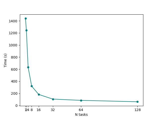
This time the code should be much faster. Once the run is over, try to run the simulation also on 32 and 64 MPI tasks. Each time, change ntasks-per-node to this number. Finally, you can try to produce a scaling plot.
The timings are contained in the r-* report files. You can already have a look at them typing
grep Time-Profile run_MPI*/r-*
The python script [parse_ytiming.py](https://hackmd.io/@palful/HkU0xblHj#parse_ytiming.py) is useful for the post-processing of report files. You can already find it in the directory, together with the reports for the longer calculations with 1, 2, 4 and 8 MPI tasks which have been provided.
If you didn't do so already, load the python module ???? ``` module purge module load matplotlib/3.2.1-foss-2020a-Python-3.8.2 ```
Then, after your jobs have finished, run the script as
```
python parse_ytiming.py run_MPI
```
to look for a report file in each run_MPI*.out folder. Make sure you have only one report file per folder.
You can also play with the script to make it print detailed timing information, however you should already see that it produced a png plot showing times-to-completion on y axis against number of MPI tasks on the x axis.
What can we learn from this plot? In particular, try to answer the following questions:
- Up to which number of MPI tasks our system efficiently scales? At which point adding more threads starts to become a waste of resources?
- How could we change our parallelisation strategy to improve the scaling even more?
- info
Keep in mind that the MPI scaling we are seeing here is not the true yambo scaling, but depends on the small size of our tutorial system. In a realistic calculation for a large-sized system, yambo has been shown to scale well up to tens of thousands of MPI tasks!
Hybrid parallelization strategy
It turns out that for this system it's not a good idea to use more than 32 MPI tasks. But we still have 128 CPUs available for this run. How to optimize the calaculation even more? We can try using OpenMP threads.
This is turned on by modifying cpus-per-task in the submission file. The product of the number of OpenMP threads and MPI tasks is equal to the total number of CPUs.
Therefore, we can distribute 128 cpus with 32 MPI tasks (efficient MPI scaling, see above) and then use 4 OpenMP threads:
#!/bin/bash
#SBATCH --nodes=1
#SBATCH --ntasks-per-node=32
#SBATCH --cpus-per-task=4
Actually, we don't need to change the related openMP variables for the yambo input, since the value 0 means "use the value of OMP_NUM_THREADS" and we have now set this environment variable to 4 via our script.
Otherwise, any positive number can directly specify the number of threads to be used in each section of the code.
DIP_Threads=  0     # [OPENMP/X] Number of threads for dipoles
...
X_Threads=  0       # [OPENMP/X] Number of threads for response functions
...
SE_Threads=  0      # [OPENMP/GW] Number of threads for self-energy
You can try to run this calculation and check if it is faster than the pure 128 MPI one from before.
You should find a massive gain: in our case, the pure MPI128_OMP1 took 01m-02s (to be changed), while the hybrid MPI32_OMP4 took (to be changed) just 37s, a 40% speedup.
You can also try any other thread combinations including the pure openMP scaling, and compare the timings.
- info
- In real-life calculations running on ncores > 100, as we have seen, it may be a good idea to adopt a hybrid approach.
- The most efficient scaling can depend both on your system and on the HPC facility you're running on. For a full CPU node on Vega (256 cores), using a large-scale system, we have found that 16 tasks times 16 threads gives the best performance.
- OpenMP can help lower memory requirements within a node. You can try to increase the OpenMP share of threads if getting Out Of Memory errors.
As mentioned above, we can conclude that the "best" parallelisation strategy is in general both system-dependent and cluster-dependent. If working on massive systems, it may be well worth your while to do preliminary parallel tests in order to work out the most efficient way to run these jobs.
[OPTIONAL] Comparing different parallelisation schemes
Up to now we always parallelised over a single parameter, i.e. c or qp. However, Yambo allows for tuning the parallelisation scheme over several parameters broadly corresponding to "loops" (i.e., summations or discrete integrations) in the code.
To this end you can open again the run_parallel.sh script and modify the section where the yambo input variables are set.
For example, X_CPU sets how the MPI Tasks are distributed in the calculation of the response function. The possibilities are shown in the X_ROLEs. The same holds for SE_CPU and SE_ROLEs which control how MPI Tasks are distributed in the calculation of the self-energy.
X_CPU= "1 1 1 $ncpu 1"      # [PARALLEL] CPUs for each role
X_ROLEs= "q g k c v"        # [PARALLEL] CPUs roles (q,g,k,c,v)
X_nCPU_LinAlg_INV= $ncpu    # [PARALLEL] CPUs for Linear Algebra
X_Threads=  0               # [OPENMP/X] Number of threads for response functions
DIP_Threads=  0             # [OPENMP/X] Number of threads for dipoles
SE_CPU= "1 $ncpu 1"         # [PARALLEL] CPUs for each role
SE_ROLEs= "q qp b"          # [PARALLEL] CPUs roles (q,qp,b)
SE_Threads=  0              # [OPENMP/GW] Number of threads for self-energy
You can try different parallelization schemes and check the performances of Yambo. In doing so, you should also change the jobname label=MPI${ncpu}_OMP${nthreads} in the run_parallel.sh script to avoid confusion with previous calculations.
You may then check how speed, memory and load balance between the CPUs are affected. You could modify the script [`parse_ytiming.py`](https://hackmd.io/@palful/HkU0xblHj#parse_ytiming.py) to parse the new data, read and distinguish between more file names, new parallelisation options, etc.
- info
- The product of the numbers entering each variable (i.e.
X_CPUandSE_CPU) times the number of threads should always match the total number of cores (unless you want to overload the cores taking advantage of multi-threads). - Using the
X_ThreadsandSE_Threadsvariables you can think about setting different hybrid schemes between the screening and the self-energy runlevels. - Memory scales better if you parallelize on bands (
c v b). - Parallelization on k-points performs similarly to parallelization on bands, but requires more memory.
- Parallelization on q-points requires much less communication between the MPI tasks. It may be useful if you run on more than one node and the inter-node connection is slow.


