Linear response from real time simulations (density matrix only)
Introduction
In this example, we will consider a single layer of hexagonal boron nitride (hBN). If you didn't before you can download input files and Yambo databases for this tutorial here: hBN-2D-RT.tar.gz. and/or follow the instructions to generate the databases here: Prerequisites for Real Time propagation with Yambo
Before proceeding with the real-time simulations it is useful to compute the Independent Particles (IP) absorption spectrum of hBN along the y direction. If you didn't before create an Inputs folder and then the input file with the commands
cd hBN-2D-RT/YAMBO/FixSymm
mkdir Inputs
yambo_rt -o c -F Inputs/01_ip.in
and set the proper input parameters
 optics                         # [R OPT] Optics
 chi                            # [R CHI] Dyson equation for Chi.
 dipoles                        # [R   ] Compute the dipoles
 Chimod= "IP"                   # [X] IP/Hartree/ALDA/LRC/PF/BSfxc
 % QpntsRXd
    1 |  1 |                   # [Xd] Transferred momenta
 %
 % BndsRnXd
   3 | 6 |                     # [Xd] Polarization function bands
 %
 % EnRngeXd
   0.00000 | 20.00000 | eV      # [Xd] Energy range
 %
 % DmRngeXd
   0.10000 |  0.10000 | eV      # [Xd] Damping range
 %
 ETStpsXd= 2001                  # [Xd] Total Energy steps
 % LongDrXd
  0.000000 | 1.000000 | 0.000000 |        # [Xd] [cc] Electric Field
 %
and then run the code
yambo_rt -F Inputs/01_ip.in -J CHI_IP -C CHI_IP
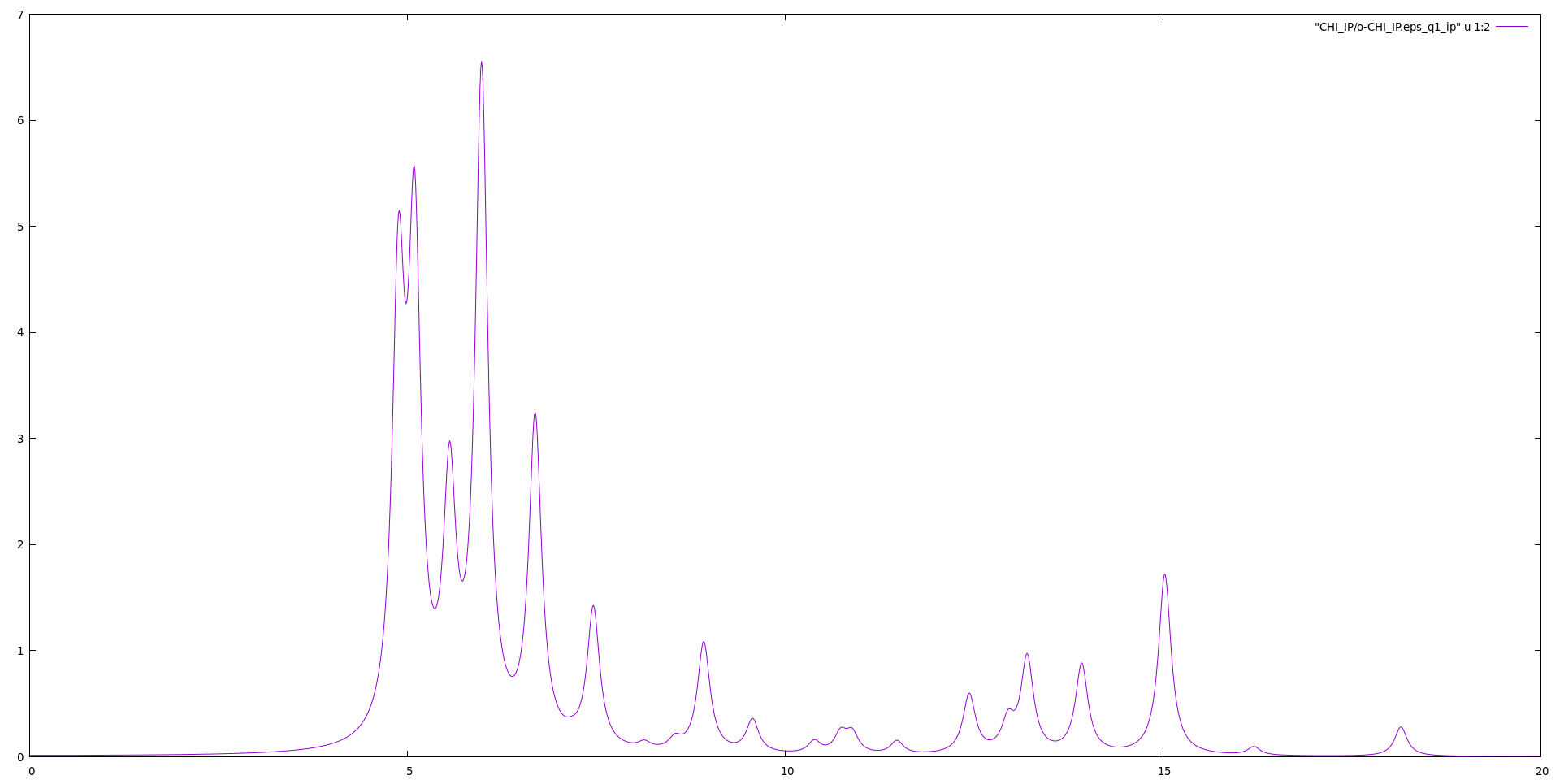
The resulting spectrum will give an idea of the energy involved in the real-time simulations
gnuplot
gnuplot> plot "CHI_IP/o-CHI_IP.eps_q1_ip" u 1:2 w l
Real-time dynamics at the independent particles level
Let us first create a folder for the input files to be run with yambo_rt.
mkdir Inputs_rt
In order to calculate linear-response in real-time, we will perturb the system with a delta function in time external field.
Use the command
yambo_rt -n p -F Inputs_rt/01_td_ip.in
to generate the input:
 negf                           # [R] Real-Time dynamics
 RT_Threads=0                   # [OPENMP/RT] Number of threads for real-time
 % RTBands
   3 |  6 |                     # [RT] Bands
 %
 Integrator= "EULER RK2"              # [RT] Integrator. Use keywords space separated  ( "EULER/EXPn/INV" "SIMPLE/RK2/RK4/HEUN" "RWA")
 PhLifeTime= 0.000000   fs      # [RT] Dephasing Time
 RTstep=10.000000       as      # [RT] Real Time step length
 NETime= 55.00000       fs      # [RT] Simulation Time
 % IOtime
  0.05     | 5.00     | 0.10     |  fs    # [RT] Time between to consecutive I/O (OBSERVABLEs,CARRIERs - GF - OUTPUT)
 %
 % Field1_Freq
  0.00     | 0.00     | eV      # [RT Field1] Frequency
 %
 Field1_Int=1.E3   kWLm2   # [RT Field1] Intensity
 Field1_Width= 0.000000 fs      # [RT Field1] Width
 Field1_kind= "DELTA"           # [RT Field1] Kind(SIN|RES|ANTIRES|GAUSS|DELTA|QSSIN)
 Field1_pol= "linear"           # [RT Field1] Pol(linear|circular)
 % Field1_Dir
  0.000000 | 1.000000 | 0.000000 |        # [RT Field1] Versor
 %
 Field1_Tstart= 0.000000fs      # [RT Field1] Initial Time
Set the field direction along y, the field type to DELTA, the length of the simulation to 55 fs, number of bands from 3 to 6, dephasing to zero and the field intensity to 1.E3 [kW/cm2].
A small intensity is needed to ensure that we remain in the perturbative regime and that the response is dominated by linear term.
The yambo_rt is optimized for TD-SEX (or even more sophisticated calculations).
Now run the simulation:
yambo_rt -F Inputs_rt/01_td_ip.in -J TD-IP_rt -C TD-IP_rt
The run produces, besides the standard report and (eventually) log files of yambo, 3 output files:
 TD-IP_rt/01_td_ip.in_TD-IP_rt
 TD-IP_rt/r-TD-IP_rt_negf
 TD-IP_rt/o-TD-IP_rt.polarization
 TD-IP_rt/o-TD-IP_rt.external_field
 TD-IP_rt/o-TD-IP_rt.current
Moreover it also makes a copy of the input file. If the run is taking to long you can open the copy of the input file TD-IP_rt/01_td_ip.in_TD-IP_rt and add there the string
STOP_NOW
It will finish the simulation in a proper way.
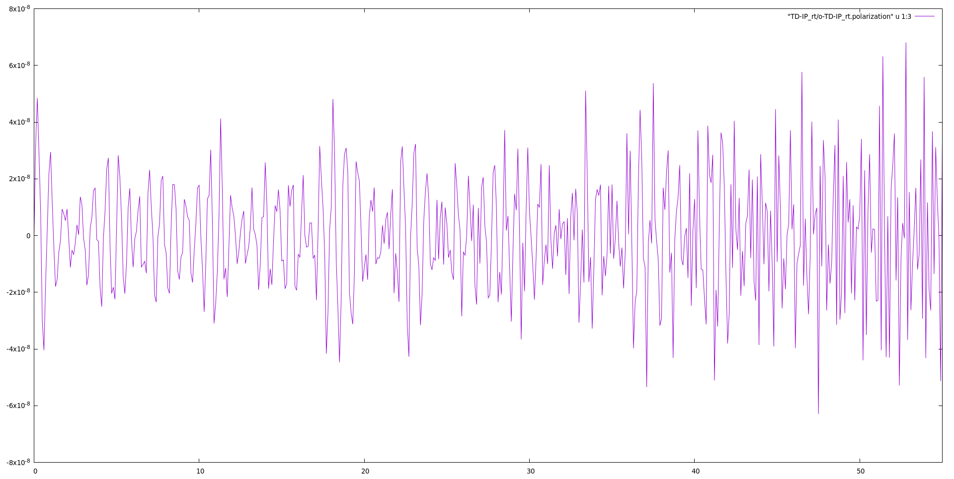
You can now plot the resulting time-dependent polarization and obtain something like this
gnuplot
plot "TD-IP_rt/o-TD-IP_rt.polarization" u 1:3 w l
The polarization is oscillating very quickly and with the time step for the output file we have chosen (100 as) we can hardly resolve the oscillations. The slowest oscillation is expected at the first absorption peak, which is located slightly above 4 eV. This corresponds to a period of about 1 fs. Higher energy transitions are however also activated by the delta like pulse, which spans all frequencies (remember that the Fourier transform of a delta function is a constant).
The I/O time, which is negligible in such calculations, is less optimized and becomes the most time demanding step here. We can overcome this setting the IOtime for the polarization to 50 as (i.e. each 5 time steps). After the run you can have a look at the timing report and you will see that indeed most of the timing was spent in the I/O:
RT databases IO : 6.8745 s CPU ( 5501 calls, 0.0012 s avg)
yambo_rt evaluates the coupling with the external field through the dipoles (by default computing the commutator [x,Hnl]); another approach is setting DipApproach="Covariant" in the input.
One can test the performance of different integrators. For example, by setting in input Integrator= "INV RK2", yambo_rt uses a similar integration scheme as yambo_nl (the latter is based on a Berry-phase approach).
Results Analysis
We can now proceed to the Fourier transform of the polarization to obtain the dielectric function
Approach based on the density matrix
Now we can use
ypp_rt -t X -F Inputs_rt/ypp_abs.in
to generate the input file
 RealTime                       # [R] Real-Time Post-Processing
 RT_X                           # [R] Response functions Post-Processing
 Xorder=1                       # Max order of the response/exc functions
 % EnRngeRt
  0.00     | 10.00     | eV      # Energy range
 %
 ETStpsRt=1001                     # Total Energy steps
 % TimeRange
  0.00     | 0.00     | fs      # Time-window where processing is done
 %
DampMode= "LORENTZIAN"             # Damping type ( NONE | LORENTZIAN | GAUSSIAN )
DampFactor=  0.10000   eV    # Damping parameter
where we set a Lorentzian smearing corresponding to 0.1 eV. Notice that due to the finite time of our simulation smearing is always necessary to Fourier transform the result. Then we run
ypp_rt -F Inputs_rt/ypp_abs.in -J TD-IP_rt -C TD-IP_rt
and obtain the files for the dielectric constant along with the field direction, the EELS along with the same direction, and the damped polarization.
o-TD-IP_rt.YPP-eps_along_E
o-TD-IP_rt.YPP-eels_along_E
o-TD-IP_rt.YPP-polarization
o-TD-IP_rt.YPP-current
o-TD-IP_rt.YPP-E_frequency
inside the folder TD-IP_rt
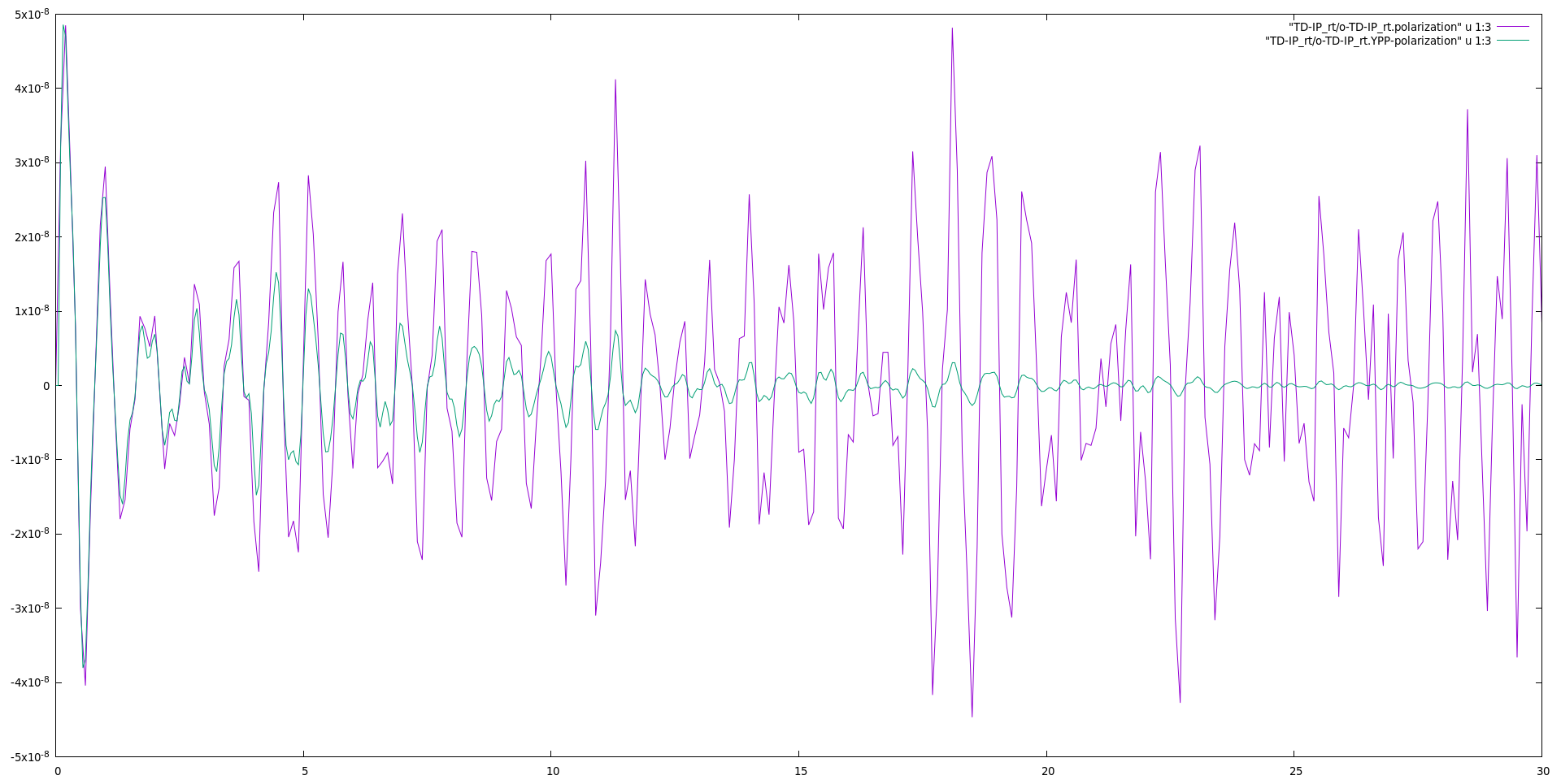
First let's have a look to the polarization.
gnuplot
plot "TD-IP_rt/o-TD-IP_rt.polarization" u 1:3 w l
replot "TD-IP_rt/o-TD-IP_rt.YPP-polarization" u 1:3 w l
We clearly see the effect of the Lorentzian damping added to the time dependent polarization
Now we can plot the dielectric constant and compare it with the linear response:


