First steps: walk through from DFT to RPA (standalone)
In this tutorial you will learn how to calculate optical spectra using Yambo, starting from a DFT calculation and ending with a look at local field effects in the optical response.
System characteristics
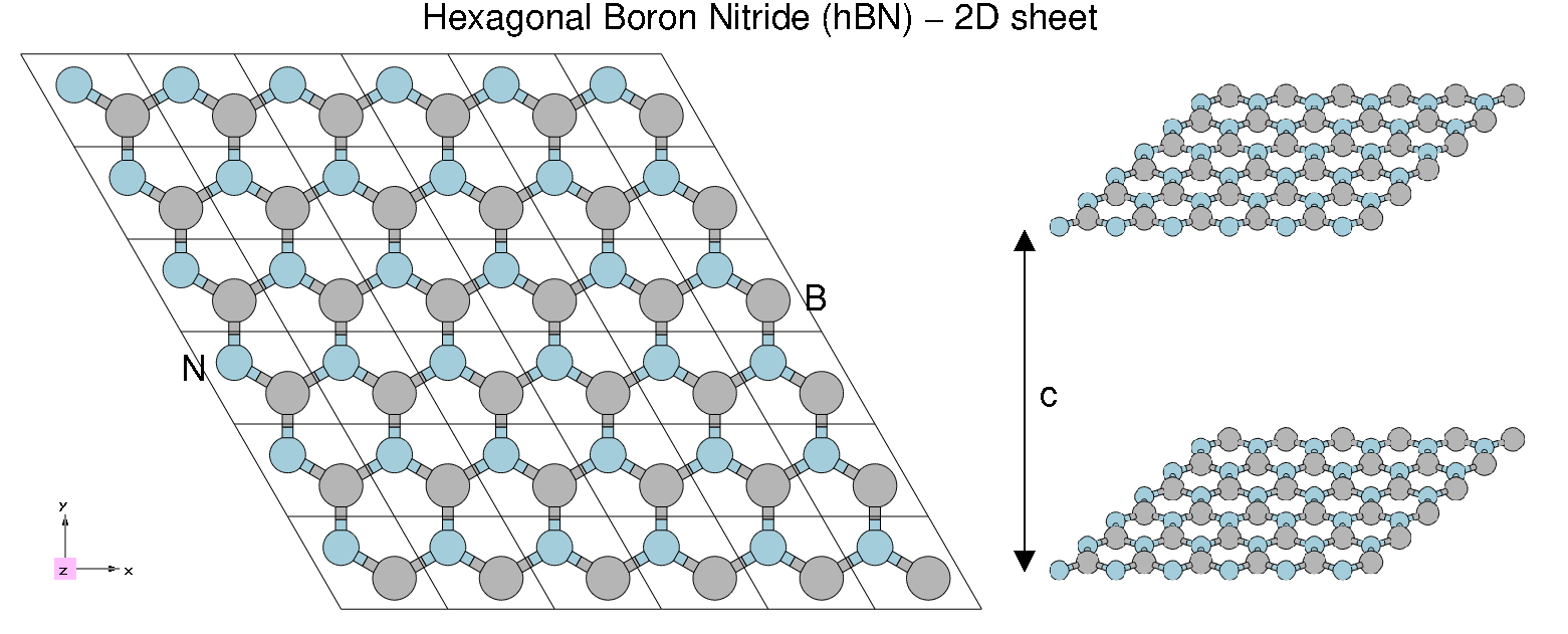
We will use a 3D system (bulk hBN) and a 2D system (hBN sheet).
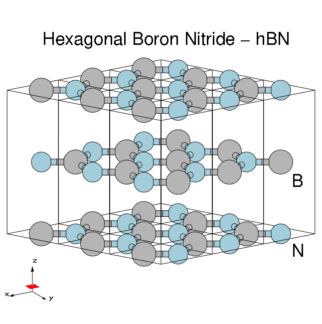
Hexagonal boron nitride - hBN:
- HCP lattice, ABAB stacking
- Four atoms per cell, B and N (16 electrons)
- Lattice constants: a = 4.716 [a.u.], c/a = 2.582
- Plane wave cutoff 40 Ry (~1500 RL vectors in wavefunctions)
- SCF run: shifted 6x6x2 grid (12 k-points) with 8 bands
- Non-SCF run: gamma-centred 6x6x2 (14 k-points) grid with 100 bands
Prerequisites
You will need:
- PWSCF input files and pseudopotentials for hBN bulk
pw.xexecutable, version 5.0 or laterp2yandyamboexecutablesgnuplotfor plotting spectra
Download the Files
Download and unpack the followint files:
hBN.tar.gz [237 MB]
hBN-2D.tar.gz [8,6 MB]
After downloading the tar.gz files just unpack them in the YAMBO_TUTORIALS folder. For example
$ mkdir YAMBO_TUTORIALS
$ mv hBN.tar.gz YAMBO_TUTORIALS
$ cd YAMBO_TUTORIALS
$ tar -xvfz hBN.tar.gz
$ ls YAMBO_TUTORIALS
  hBN
(Advanced users can download and install all tutorial files using git. See the main Tutorial Files page.)
DFT calculation of bulk hBN and conversion to Yambo
In this module you will learn how to generate the Yambo SAVE folder for bulk hBN starting from a PWscf calculation.
DFT calculations
$ cd YAMBO_TUTORIALS/hBN/PWSCF
$ ls
Inputs		Pseudos		PostProcessing		References
hBN_scf.in	hBN_nscf.in     hBN_scf_plot_bands.in  hBN_nscf_plot_bands.in
First run the SCF calculation to generate the ground-state charge density, occupations, Fermi level, and so on:
$ pw.x < hBN_scf.in > hBN_scf.out
Inspection of the output shows that the valence band maximum lies at 5.06eV.
Next run a non-SCF calculation to generate a set of Kohn-Sham eigenvalues and eigenvectors for both occupied and unoccupied states (100 bands):
$ pw.x < hBN_nscf.in > hBN_nscf.out                  (serial run, ~1 min) OR
$ mpirun -np 2 pw.x < hBN_nscf.in > hBN_nscf.out       (parallel run, 40s)
Here we use a 6x6x2 grid giving 14 k-points, but denser grids should be used for checking convergence of Yambo runs.
Note the presence of the following flags in the input file:
wf_collect=.true.
force_symmorphic=.true.
diago_thr_init=5.0e-6,
diago_full_acc=.true.
which are needed for generating the Yambo databases accurately. Full explanations of these variables are given on the quantum-ESPRESSO input variables page.
After these two runs, you should have a hBN.save directory:
$ ls hBN.save
data-file.xml charge-density.dat gvectors.dat B.pz-vbc.UPF N.pz-vbc.UPF
K00001	K00002 .... 	K00035	K00036
Conversion to Yambo format
The PWscf bBN.save output is converted to the Yambo format using the p2y executable (pwscf to yambo), found in the yambo bin directory.
Enter hBN.save and launch p2y:
$ cd hBN.save
$ p2y
...
<---> DBs path set to .
<---> Index file set to data-file.xml
<---> Header/K-points/Energies... done
...
<---> == DB1 (Gvecs and more) ...
<---> ... Database done
<---> == DB2 (wavefunctions)  ... done ==
<---> == DB3 (PseudoPotential) ... done ==
<--->  == P2Y completed ==
This output repeats some information about the system and generates a SAVE directory:
$ ls SAVE
ns.db1  ns.wf  ns.kb_pp_pwscf
ns.wf_fragments_1_1 ...
ns.kb_pp_pwscf_fragment_1 ...
These files, with an n prefix, indicate that they are in netCDF format, and thus not human readable. However, they are perfectly transferable across different architectures. You can check that the databases contain the information you expect by launching Yambo using the -D option:
$ yambo -D
[RD./SAVE//ns.db1]------------------------------------------
Bands                           : 100
K-points                        : 14
G-vectors             [RL space]:  8029
Components       [wavefunctions]: 1016
...
[RD./SAVE//ns.wf]-------------------------------------------
Fragmentation                    :yes
...
[RD./SAVE//ns.kb_pp_pwscf]----------------------------------
Fragmentation                    :yes
- S/N 006626 -------------------------- v.04.01.02 r.00000 -
In practice we suggest to move the SAVE folder into a new clean folder.
In this tutorial however, we ask instead that you continue using a SAVE folder that we prepared previously:
$ cd ../../YAMBO
$ ls
SAVE
Initialization of Yambo databases
Use the SAVE folders that are already provided, rather than any ones you may have generated previously.
Every Yambo run must start with this step. Go to the folder containing the hBN-bulk SAVE directory:
$ cd YAMBO_TUTORIALS/hBN/YAMBO
$ ls
SAVE
and simply launch the code
$ yambo
This will run the initialization (setup) runlevel.
TIP: do not run yambo from inside the SAVE folder! In fact, if you ever see the message:
yambo: cannot access CORE database (SAVE/*db1 and/or SAVE/*wf)
it usually means you are trying to launch Yambo from the wrong place.
Three new elements will appear:
Run-time output
This is typically written to standard output (on screen) and tracks the progress of the run in real time:
<---> [01] CPU structure, Files & I/O Directories
<---> [02] CORE Variables Setup
<---> [02.01] Unit cells
<---> [02.02] Symmetries
<---> [02.03] RL shells
<---> Shells finder |########################################| [100%] --(E) --(X)
<---> [02.04] K-grid lattice
<---> [02.05] Energies [ev] & Occupations
<---> [03] Transferred momenta grid
<---> BZ -> IBZ reduction |########################################| [100%] --(E) --(X)
<---> X indexes |########################################| [100%] --(E) --(X)
<---> SE indexes |########################################| [100%] --(E) --(X)
<---> [04] External corrections
<---> [05] Game Over & Game summary
Specific runlevels are indicated with numeric labels like [02.02].
The hashes (#) indicate progress of the run in Wall Clock time, indicating the elapsed (E) and expected (X) time to complete a runlevel, and the percentage of the task complete.
If Yambo is launched using a script, or as a background process, or in parallel, this output will appear in a log file prefixed by the letter l, in this case as l_setup.
If this log file already exists from a previous run, it will not be overwritten. Instead, a new file will be created with an incrementing numerical label, e.g. l_setup_01, l_setup_02, etc. This applies to all files created by Yambo.
In the case of parallel runs, CPU-dependent log files will appear inside a LOG folder, e.g.
$ mpirun -np 4 yambo
$ ls LOG
l_setup_CPU_1   l_setup_CPU_2  l_setup_CPU_3  l_setup_CPU_4
This behaviour can be controlled at runtime - see the Parallel tutorial for details.
New core databases
New databases appear in the SAVE folder:
$ ls SAVE
ns.db1 ns.wf ns.kb_pp_pwscf ndb.gops ndb.kindx
ns.wf_fragments_1_1 ...
ns.kb_pp_pwscf_fragment_1 ...
These contain information about the G-vector shells and k/q-point meshes as defined by the DFT calculation.
In general: a database called ns.xxx is a static database, generated once by p2y, while databases called ndb.xxx are dynamically generated while you use yambo.
TIP: if you launch yambo, but it does not seem to do anything, check that these files are present.
Report file
A report file r_setup is generated in the run directory. This mostly reports information about the ground state system as defined by the DFT run, but also adds information about the band gaps, occupations, shells of G-vectors, IBZ/BZ grids, the CPU structure (for parallel runs), and so on. Some points of note:
 [02.03] RL shells
 =================
 Shells, format: [S#] G_RL(mHa)
  [S453]:8029(0.7982E+5) [S452]:8005(0.7982E+5) [S451]:7981(0.7982E+5) [S450]:7957(0.7942E+5)
  ...
  [S4]:11( 1183.) [S3]:5( 532.5123) [S2]:3( 133.1281) [S1]:1( 0.000000)
This reports the set of closed reciprocal lattice (RL) shells defined internally that contain G-vectors with the same modulus. The highest number of RL vectors we can use is 8029. Yambo will always redefine any input variable in RL units to the nearest closed shell.
 [02.05] Energies [ev] & Occupations
 ===================================
 Fermi Level        [ev]:  5.112805
 VBM / CBm          [ev]:  0.000000  3.876293
 Electronic Temp. [ev K]:  0.00      0.00
 Bosonic    Temp. [ev K]:  0.00      0.00
 El. density      [cm-3]: 0.460E+24
 States summary         : Full        Metallic    Empty
                          0001-0008               0009-0100
 Indirect Gaps      [ev]: 3.876293  7.278081
 Direct Gaps        [ev]:  4.28829  11.35409
 X BZ K-points :  72
Yambo recalculates again the Fermi level (close to the value of 5.06 noted in the PWscf SCF calculation). From here on, however, the Fermi level is set to zero, and other eigenvalues are shifted accordingly. The system is insulating (8 filled, 92 empty) with an indirect band gap of 3.87 eV. The minimum and maximum direct and indirect gaps are indicated. There are 72 k-points in the full BZ, generated using symmetry from the 14 k-points in our user-defined grid.
TIP: You should inspect the report file after every run for errors and warnings.
2D hBN
Simply repeat the steps above. Go to the folder containing the hBN-sheet SAVE directory and launch yambo:
$ cd TUTORIALS/hBN-2D/YAMBO
$ ls
SAVE
$ yambo
Again, inspect the r_setup file, output logs, and verify that ndb.gops and ndb.kpts have been created inside the SAVE folder.
You are now ready to use Yambo!
Yambo's command line interface
Yambo uses a command line interface to select tasks, generate input files, and control the runtime behaviour.
In this module you will learn how to select tasks, generate and modify input files, and control the runtime behaviour by using Yambo's command line interface.
Command line options are divided into uppercase and lowercase options:
- Lowercase: select tasks, generate input files, and (by default) launch a file editor
- Uppercase: modify Yambo's default settings, at run time and when generating input files
Lowercase and uppercase options can be used together.
Input file generator
First, move to the appropriate folder and initialize the Yambo databases if you haven't already done so.
$ cd YAMBO_TUTORIALS/hBN/YAMBO
$ yambo                    (initialize)
Yambo generates its own input files: you just tell the code what you want to calculate by launching Yambo along with one or more lowercase options.
Allowed options
To see the list of runlevels and options, run yambo -h or better,
$ yambo -H
This is yambo 4.4.0 rev.148
A shiny pot of fun and happiness [C.D.Hogan]
-h		:Short Help
-H		:Long Help
-J <opt>	:Job string identifier
-V <opt>	:Input file verbosity[opt=RL,kpt,sc,qp,io,gen,resp,all,par]
-F <opt>	:Input file
-I <opt>	:Core I/O directory
-O <opt>	:Additional I/O directory
-C <opt>	:Communications I/O directory
-D		:DataBases properties
-W <opt>	:Wall Time limitation (1d2h30m format)
-Q		:Don't launch the text editor
-E <opt>	:Environment Parallel Variables file
-M		:Switch-off MPI support (serial run)
-N		:Switch-off OpenMP support (single thread run)
-i		:Initialization
-o <opt>	:Optics [opt=(c)hi is (G)-space / (b)se is (eh)-space ]
-k <opt>	:Kernel [opt=hartree/alda/lrc/hf/sex](hf/sex only eh-space; lrc only G-space)
-y <opt>	:BSE solver [opt=h/d/s/(p/f)i](h)aydock/(d)iagonalization/(i)nversion
-r		:Coulomb potential
-x		:Hartree-Fock Self-energy and local XC
-d		:Dynamical Inverse Dielectric Matrix
-b		:Static Inverse Dielectric Matrix
-p <opt>	:GW approximations [opt=(p)PA/(c)HOSEX]
-g <opt>	:Dyson Equation solver[opt=(n)ewton/(s)ecant/(g)reen]
-l		:GoWo Quasiparticle lifetimes
-a		:ACFDT Total Energy
-s		:ScaLapacK test
Any time you launch Yambo with a lowercase option, Yambo will generate the appropriate input file (default name: yambo.in) and launch the vi editor.
Editor choice can be changed at configure; alternatively you can use the -Q run time option to skip the automatic editing (do this if you are not familiar with vi!):
$ yambo -x -Q
yambo: input file yambo.in created
$ emacs yambo.in     or your favourite editing tool
Combining options
Multiple options can be used together to activate various tasks or runlevels (in some cases this is actually a necessity). For instance, to generate an input file for optical spectra including local field effects (Hartree approximation), do (and then exit)
$ yambo -o c -k hartree       which switches on:
optics                       # [R OPT] Optics
chi                          # [R CHI] Dyson equation for Chi.
Chimod= "Hartree"            # [X] IP/Hartree/ALDA/LRC/BSfxc
To perform a Hartree-Fock and GW calculation using a plasmon-pole approximation, do (and then exit):
$ yambo -x -g n -p p        which switches on:
HF_and_locXC                 # [R XX] Hartree-Fock Self-energy and Vxc
gw0                          # [R GW] GoWo Quasiparticle energy levels
ppa                          # [R Xp] Plasmon Pole Approximation
em1d                         # [R Xd] Dynamical Inverse Dielectric Matrix
Each runlevel activates its own list of variables and flags.
Changing input parameters
Yambo reads various parameters from existing database files and/or input files and uses them to suggest values or ranges. Let's illustrate this by generating the input file for a Hartree-Fock calculation.
$ yambo -x
Inside the generated input file you should find:
EXXRLvcs =  3187        RL    # [XX] Exchange RL components
%QPkrange                    # [GW] QP generalized Kpoint/Band indices
  1| 14|  1|100|
%
The QPkrange variable (follow the link for a "detailed" explanation for any variable) suggests a range of k-points (1 to 14) and bands (1 to 100) based on what it finds in the core database SAVE/ns.db1, i.e. as defined by the DFT code.
Leave that variable alone, and instead modify the previous variable to EXXRLvcs= 1000 RL
Save the file, and now generate the input a second time with yambo -x. You will see:
EXXRLvcs= 1009 RL
This indicates that Yambo has read the new input value (1000 G-vectors), checked the database of G-vector shells (SAVE/ndb.gops), and changed the input value to one that fits a completely closed shell.
Last, note that Yambo variables can be expressed in different units. In this case, RL can be replaced by an energy unit like Ry, eV, Ha, etc. Energy units are generally better as they are independent of the cell size. Technical information is available on the Variables page.
The input file generator of Yambo is thus an intelligent parser, which interacts with the user and the existing databases. For this reason we recommend that you always use Yambo to generate the input files, rather than making them yourself.
Uppercase options
Uppercase options modify some of the code's default settings. They can be used when launching the code but also when generating input files.
Allowed options
To see the list of options, again do:
$ yambo -H
Tool: yambo 4.1.2 rev.14024
Description: A shiny pot of fun and happiness [C.D.Hogan]
-J <opt>	:Job string identifier
-V <opt>	:Input file verbosity
                [opt=RL,kpt,sc,qp,io,gen,resp,all,par]
-F <opt>	:Input file
-I <opt>	:Core I/O directory
-O <opt>	:Additional I/O directory
-C <opt>	:Communications I/O directory
-D		:DataBases properties
-W <opt>	:Wall Time limitation (1d2h30m format)
-Q		:Don't launch the text editor
-M		:Switch-off MPI support (serial run)
-N		:Switch-off OpenMP support (single thread run)
[Lower case options]
Command line options are extremely important to master if you want to use yambo productively. Often, the meaning is clear from the help menu:
$ yambo -F yambo.in_HF -x    Make a Hartree -Fock input file called yambo.in_HF
$ yambo -D                   Summarize the content of the databases in the SAVE folder
$ yambo -I ../               Run the code, using a SAVE folder in a directory one level up
$ yambo -C MyTest            Run the code, putting all report, log, plot files inside a folder MyTest
Other options deserve a closer look.
Verbosity
Yambo uses many input variables, many of which can be left at their default values. To keep input files short and manageable, only a few variables appear by default in the inout file. More advanced variables can be switched on by using the -V verbosity option. These are grouped according to the type of variable. For instance, -V RL switches on variables related to G vector summations, and -V io switches on options related to I/O control. Try:
$ yambo -o c -V RL       switches on:
FFTGvecs=  3951        RL    # [FFT] Plane-waves

$ yambo -o c -V io       switches on:
StdoHash=  40                # [IO] Live-timing Hashes
DBsIOoff= "none"             # [IO] Space-separated list of DB with NO I/O. DB= ...
DBsFRAGpm= "none"            # [IO] Space-separated list of +DB to be FRAG and ...
#WFbuffIO                    # [IO] Wave-functions buffered I/O
Unfortunately, -V options must be invoked and changed one at a time. When you are more expert, you may go straight to -V all, which turns on all possible variables. However note that yambo -o c -V all adds an extra 30 variables to the input file, which can be confusing: use it with care.
Job script label
The best way to keep track of different runs using different parameters is through the -J flag. This inserts a label in all output and report files, and creates a new folder containing any new databases (i.e. they are not written in the core SAVE folder). Try:
$ yambo -J 1Ry -V RL -x        and modify to
FFTGvecs = 1 Ry
EXXGvecs = 1 Ry
$ yambo -J 1Ry           Run the code
$ ls
yambo.in SAVE
o-1Ry.hf r-1Ry_HF_and_locXC 1Ry 1Ry/ndb.HF_and_locXC
This is extremely useful when running convergence tests, trying out different parameters, etc.
Exercise: use yambo to report the properties of all database files (including ndb.HF_and_locXC)
Optical absorption in hBN: independent particle approximation
Background
The dielectric function in the long-wavelength limit, at the independent particle level (RPA without local fields), is essentially given by the following:
In practice, Yambo does not use this expression directly but solves the Dyson equation for the susceptibility X, which is described in the Local fields module.
Choosing input parameters
Enter the folder for bulk hBN that contains the SAVE directory, run the initialization and generate the input file. From yambo -H you should understand that the correct option is yambo -o c. Let's add some command line options:
$ cd YAMBO_TUTORIALS/hBN/YAMBO
$ yambo               (initialization)
$ yambo -F yambo.in_IP -o c
This corresponds to optical properties in G-space at the independent particle level: in the input file this is indicated by (Chimod= "IP").
Optics runlevel
For optical properties we are interested just in the long-wavelength limit q = 0. This always corresponds to the first q-point in the set of possible q=k-k' -points. Change the following variables in the input file to:
% QpntsRXd
 1 |  1 |                   # [Xd] Transferred momenta
%
ETStpsXd= 1001               # [Xd] Total Energy steps
in order to select just the first q. The last variable ensures we generate a smooth spectrum. Save the input file and launch the code, keeping the command line options as before (i.e., just remove the lower case options):
$ yambo -F yambo.in_IP -J Full
...
<---> [05] Optics
<---> [LA] SERIAL linear algebra
<---> [DIP] Checking dipoles header
<---> [x,Vnl] computed using 4 projectors
<---> [M  0.017 Gb] Alloc WF ( 0.016)
<---> [WF] Performing Wave-Functions I/O from ./SAVE
<01s> Dipoles: P and iR (T): |########################################| [100%] 01s(E) 01s(X)
<01s> [M  0.001 Gb] Free WF ( 0.016)
<01s> [DIP] Writing dipoles header
<01s> [X-CG] R(p) Tot o/o(of R)  :   5501   52992     100
<01s> Xo@q[1] |########################################| [100%] --(E) --(X)
<01s> [06] Game Over & Game summary

$ ls
Full   SAVE  yambo.in_IP   r_setup
o-Full.eel_q1_ip  o-Full.eps_q1_ip  r-Full_optics_chi
Let's take a moment to understand what Yambo has done inside the Optics runlevel:
- Compute the [x,Vnl] term
- Read the wavefunctions from disc [WF]
- Compute the dipoles, i.e. matrix elements of p
- Write the dipoles to disk as Full/ndb.dip* databases. This you can see in the report file:
$ grep -A20 "WR" r-Full_optics_chi
[WR./Full//ndb.dip_iR_and_P]
Brillouin Zone Q/K grids (IBZ/BZ):  14   72   14   72
RL vectors                   (WF): 1491
Electronic Temperature        [K]: 0.0000000
Bosonic    Temperature        [K]: 0.0000000
X band range           :   1  100
RL vectors in the sum  : 1491
[r,Vnl] included       :yes
...
- Finally, Yambo computes the non-interacting susceptibility X0 for this q, and writes the dielectric function inside the o-Full.eps_q1_ip file for plotting
Energy cut off
Before plotting the output, let's change a few more variables. The previous calculation used all the G-vectors in expanding the wavefunctions, up to 1491 (~1016 components). This corresponds roughly to the cut off energy of 40Ry we used in the DFT calculation. Generally, however, we can use a smaller value. We use the verbosity to switch on this variable, and a new -J flag to avoid reading the previous database:
$ yambo -F yambo.in_IP -J 6Ry -V RL -o c
Change the value of FFTGvecs and also its unit from RL (number of G-vectors) to Ry (energy in Rydberg):
FFTGvecs= 6 Ry # [FFT] Plane-waves
Save the input file and launch the code again:
$ yambo -F yambo.in_IP -J 6Ry
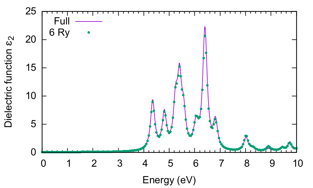
and then plot the o-Full.eps_q1_ip and o-6Ry.eps_q1_ip files:
$ gnuplot
gnuplot> plot "o-Full.eps_q1_ip" w l,"o-6Ry.eps_q1_ip" w p
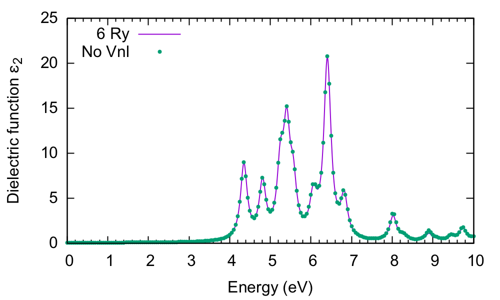
Clearly there is very little difference between the two spectra. This highlights an important point in calculating excited state properties: generally, fewer G-vectors are needed than what are needed in DFT calculations. Regarding the spectrum itself, the first peak occurs at about 4.4eV. This is consistent with the minimum direct gap reported by Yambo: 4.28eV. The comparison with experiment (not shown) is very poor however.
If you make some mistake, and cannot reproduce this figure, you should check the value of FFTGvecs in the input file, delete the 6Ry folder, and try again - taking care to plot the right file! (e.g. o-6Ry.eps_q1_ip_01).
q-direction
Now let's select a different component of the dielectric tensor:
$ yambo -F yambo.in_IP -J 6Ry -V RL -o c
...
% LongDrXd
0.000000 | 0.000000 | 1.000000 |        # [Xd] [cc] Electric Field
%
...
$ yambo -F yambo.in_IP -J 6Ry
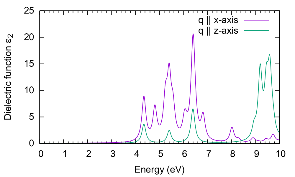
This time yambo reads from the 6Ry folder, so it does not need to compute the dipole matrix elements again, and the calculation is fast. Plotting gives:
$ gnuplot
gnuplot> plot "o-6Ry.eps_q1_ip" t "q || x-axis" w l,"o-6Ry.eps_q1_ip_01" t "q || c-axis" w l
The absorption is suppressed in the stacking direction. As the interplanar spacing is increased, we would eventually arrive at the absorption of the BN sheet (see Local fields tutorial).
Non-local commutator
Last, we show the effect of switching off the non-local commutator term (see [Vnl,r] in the equation at the top of the page) due to the pseudopotential. As there is no option to do this inside yambo, you need to hide the database file. Change back to the q || (1 0 0) direction, and launch yambo with a different -J option:
$ mv SAVE/ns.kb_pp_pwscf SAVE/ns.kb_pp_pwscf_OFF
$ yambo -F yambo.in_IP -J 6Ry_NoVnl -o c             (change to q || 100)
$ yambo -F yambo.in_IP -J 6Ry_NoVnl
Note the warning in the output:
<---> [WARNING] Missing non-local pseudopotential contribution
which also appears in the report file, and noted in the database as [r,Vnl] included :no. The difference is tiny:
However, when your system is larger, with more projectors in the pseudopotential or more k-points (see the BSE tutorial), the inclusion of Vnl can make a huge difference in the computational load, so it's always worth checking to see if the terms are important in your system.
Optical absorption in 2D BN: local field effects
Background
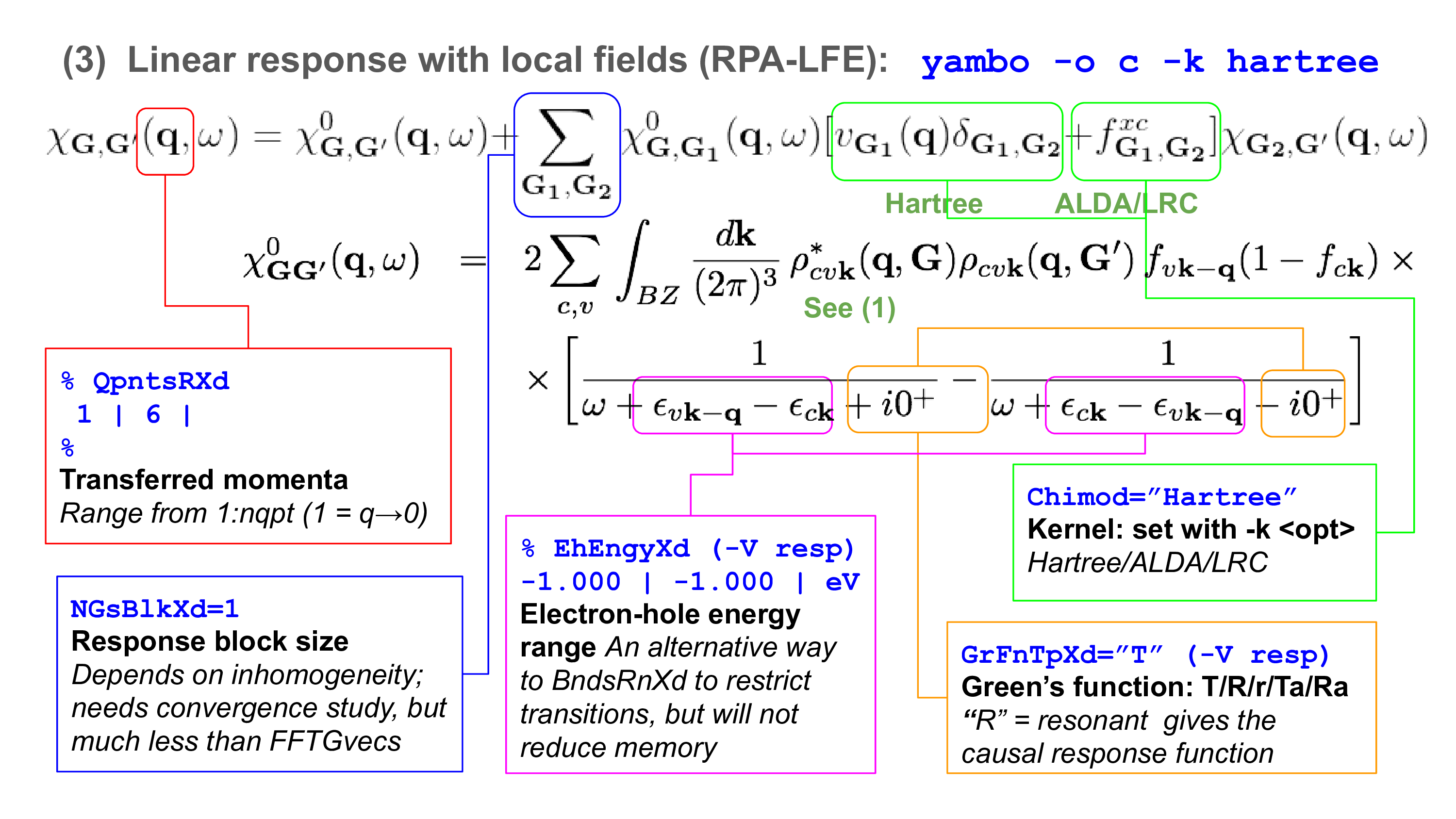
The macroscopic dielectric function is obtained by including the so-called local field effects (LFE) in the calculation of the response function. Within the time-dependent DFT formalism this is achieved by solving the Dyson equation for the susceptibility X. In reciprocal space this is given by:
The microscopic dielectric function is related to X by:
and the macroscopic dielectric function is obtained by taking the (0,0) component of the inverse microscopic one:
Experimental observables like the optical absorption and the electron energy loss can be obtained from the macroscopic dielectric function:
In the following we will neglect the f xc term: we perform the calculation at the RPA level and consider just the Hartree term (from vG) in the kernel. If we also neglect the Hartree term, we arrive back at the independent particle approximation, since there is no kernel and X = X0.
Choosing input parameters
Enter the folder for 2D hBN that contains the SAVE directory, and generate the input file. From yambo -H you should understand that the correct option is yambo -o c -k hartree. Let's start by running the calculation for light polarization q in the plane of the BN sheet:
$ cd YAMBO_TUTORIALS/hBN-2D/YAMBO
$ yambo        (Initialization)
$ yambo -F yambo.in_RPA -V RL -J q100 -o c -k hartree
We thus use a new input file yambo.in_RPA, switch on the FFTGvecs variable, and label all outputs/databases with a q100 tag. Make sure to set/modify all of the following variables to:
FFTGvecs=     6        Ry    # [FFT] Plane-waves
Chimod= "Hartree"            # [X] IP/Hartree/ALDA/LRC/BSfxc
NGsBlkXd=     3        Ry    # [Xd] Response block size
% QpntsRXd
 1 |  1 |                   # [Xd] Transferred momenta
%
% EnRngeXd
 0.00000 | 20.00000 | eV    # [Xd] Energy range
%
% DmRngeXd
0.200000 | 0.200000 | eV    # [Xd] Damping range
%
ETStpsXd= 2001               # [Xd] Total Energy steps
% LongDrXd
1.000000 | 0.000000 | 0.000000 |        # [Xd] [cc] Electric Field
%
In this input file, we have:
- A q parallel to the sheet
- A wider energy range than before, and more broadening
- Selected the Hartree kernel, and expanded G-vectors in the screening up to 3 Ry (about 85 G-vectors)
LFEs in periodic direction
Now let's run the code with this new input file (CECAM in serial: about 2mins; parallel 4 tasks: 50s)
$ yambo -F yambo.in_RPA -J q100
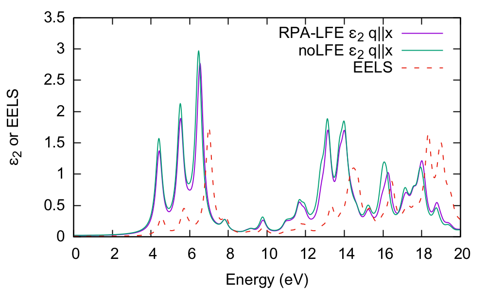
and let's compare the absorption with and without the local fields included. By inspecting the o-q100.eps_q1_inv_rpa_dyson file we find that this information is given in the 2nd and 4th columns, respectively:
$ head -n30 o-q100.eps_q1_inv_rpa_dyson
# Absorption @ Q(1) [q->0 direction] : 1.0000000  0.0000000  0.0000000
#  E/ev[1]     EPS-Im[2]   EPS-Re[3]   EPSo-Im[4]  EPSo-Re[5]
Plot the result:
$ gnuplot
gnuplot> plot "o-q100.eps_q1_inv_rpa_dyson" u 1:2 w l,"o-q100.eps_q1_inv_rpa_dyson" u 1:4 w l
It is clear that there is little influence of local fields in this case. This is generally the case for semiconductors or materials with a smoothly varying electronic density. We have also shown the EELS spectrum (o-q100.eel_q1_inv_rpa_dyson) for comparison.
LFEs in non-periodic direction
Now let's switch to q perpendicular to the BN plane:
$ yambo -F yambo.in_RPA -V RL -o c -k hartree        and set
...
% LongDrXd
0.000000 | 0.000000 | 1.000000 |        # [Xd] [cc] Electric Field
%
You can try out the default parallel usage now, or run again in serial, i.e.
$ yambo -F yambo.in_RPA  -J q001       (serial)
$ mpirun -np 4 yambo -F yambo.in_RPA  -J q001 &      (parallel, MPI only, 4 tasks)
As noted previously, the log files in parallel appear in the LOG folder, you can follow the execution with tail -F LOG/l-q001_optics_chi_CPU_1 .
Plotting the output file:
$ gnuplot
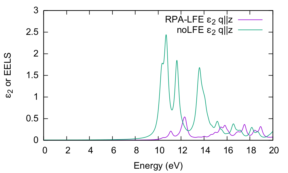
gnuplot> plot "o-q001.eps_q1_inv_rpa_dyson" u 1:2 w l,"o-q001.eps_q1_inv_rpa_dyson" u 1:4 w l
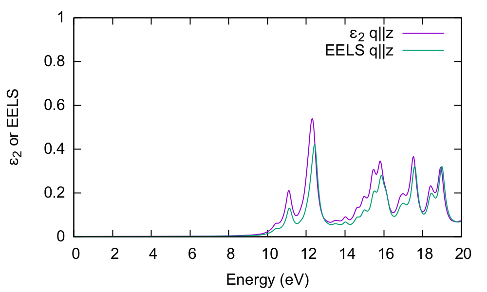
In this case, the absorption is strongly blueshifted with respect to the in-plane absorption. Furthermore, the influence of local fields is striking, and quenches the spectrum strongly. This is the well known depolarization effect. Local field effects are much stronger in the perpendicular direction because the charge inhomogeneity is dramatic. Many G-vectors are needed to account for the sharp change in the potential across the BN-vacuum interface.
Absorption versus EELS
In order to understand this further, we plot the electron energy loss spectrum for this component and compare with the absorption:
$ gnuplot
gnuplot > plot "o-q001.eps_q1_inv_rpa_dyson" w l,"o-q001.eel_q1_inv_rpa_dyson" w l
The conclusion is that the absorption and EELS coincide for isolated systems. To understand why this is, you need to consider the role of the macroscopic screening in the response function and the long-range part of the Coulomb potential. See e.g.[1]
- ↑ TDDFT from molecules to solids: The role of long‐range interactions, F. Sottile et al, International journal of quantum chemistry 102 (5), 684-701 (2005)
