First steps: walk through from DFT to RPA (standalone)
In this tutorial you will learn how to calculate optical spectra using Yambo, starting from a DFT calculation and ending with a look at local field effects in the optical response.
System characteristics
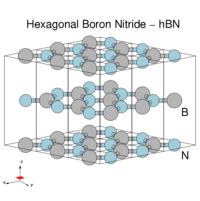
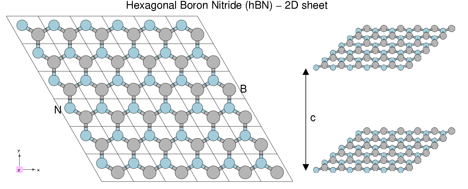
We will use a 3D system (bulk hBN) and a 2D system (hBN sheet).
Hexagonal boron nitride - hBN:
- HCP lattice, ABAB stacking
- Four atoms per cell, B and N (16 electrons)
- Lattice constants: a = 4.716 [a.u.], c/a = 2.582
- Plane wave cutoff 40 Ry (~1500 RL vectors in wavefunctions)
- SCF run: shifted 6x6x2 grid (12 k-points) with 8 bands
- Non-SCF run: gamma-centred 6x6x2 (14 k-points) grid with 100 bands
Prerequisites
You will need:
- PWSCF input files and pseudopotentials for hBN bulk
pw.xexecutable, version 5.0 or laterp2yandyamboexecutables
Step 0: Download the Files
Download and unpack the hBN.tar.gz and hBN-2D.tar.gz files. After downloading the tar.gz files just unpack them in the YAMBO_TUTORIALS folder. For example
$ mkdir YAMBO_TUTORIALS
$ mv hBN.tar.gz YAMBO_TUTORIALS
$ cd YAMBO_TUTORIALS
$ tar -xvfz hBN.tar.gz
$ ls YAMBO_TUTORIALS
  hBN
(Advanced users can download and install all tutorial files using git. See the main Tutorial Files page.)
Step 1: DFT calculation of bulk hBN and conversion to Yambo
In this module you will learn how to generate the Yambo SAVE folder for bulk hBN starting from a PWscf calculation.
DFT calculations
$ cd YAMBO_TUTORIALS/hBN/PWSCF
$ ls
Inputs		Pseudos		PostProcessing		References
hBN_scf.in	hBN_nscf.in     hBN_scf_plot_bands.in  hBN_nscf_plot_bands.in
First run the SCF calculation to generate the ground-state charge density, occupations, Fermi level, and so on:
$ pw.x < hBN_scf.in > hBN_scf.out
Inspection of the output shows that the valence band maximum lies at 5.06eV.
Next run a non-SCF calculation to generate a set of Kohn-Sham eigenvalues and eigenvectors for both occupied and unoccupied states (100 bands):
$ pw.x < hBN_nscf.in > hBN_nscf.out                  (serial run, ~1 min) OR
$ mpirun -np 2 pw.x < hBN_nscf.in > hBN_nscf.out       (parallel run, 40s)
Here we use a 6x6x2 grid giving 14 k-points, but denser grids should be used for checking convergence of Yambo runs.
Note the presence of the following flags in the input file:
wf_collect=.true.
force_symmorphic=.true.
diago_thr_init=5.0e-6,
diago_full_acc=.true.
which are needed for generating the Yambo databases accurately. Full explanations of these variables are given on the quantum-ESPRESSO input variables page.
After these two runs, you should have a hBN.save directory:
$ ls hBN.save
data-file.xml charge-density.dat gvectors.dat B.pz-vbc.UPF N.pz-vbc.UPF
K00001	K00002 .... 	K00035	K00036
Conversion to Yambo format
The PWscf bBN.save output is converted to the Yambo format using the p2y executable (pwscf to yambo), found in the yambo bin directory.
Enter hBN.save and launch p2y:
$ cd hBN.save
$ p2y
...
<---> DBs path set to .
<---> Index file set to data-file.xml
<---> Header/K-points/Energies... done
...
<---> == DB1 (Gvecs and more) ...
<---> ... Database done
<---> == DB2 (wavefunctions)  ... done ==
<---> == DB3 (PseudoPotential) ... done ==
<--->  == P2Y completed ==
This output repeats some information about the system and generates a SAVE directory:
$ ls SAVE
ns.db1  ns.wf  ns.kb_pp_pwscf
ns.wf_fragments_1_1 ...
ns.kb_pp_pwscf_fragment_1 ...
These files, with an n prefix, indicate that they are in netCDF format, and thus not human readable. However, they are perfectly transferable across different architectures. You can check that the databases contain the information you expect by launching Yambo using the -D option:
$ yambo -D
[RD./SAVE//ns.db1]------------------------------------------
Bands                           : 100
K-points                        : 14
G-vectors             [RL space]:  8029
Components       [wavefunctions]: 1016
...
[RD./SAVE//ns.wf]-------------------------------------------
Fragmentation                    :yes
...
[RD./SAVE//ns.kb_pp_pwscf]----------------------------------
Fragmentation                    :yes
- S/N 006626 -------------------------- v.04.01.02 r.00000 -
In practice we suggest to move the SAVE folder into a new clean folder.
In this tutorial however, we ask instead that you continue using a SAVE folder that we prepared previously:
$ cd ../../YAMBO
$ ls
SAVE
Summary
From this tutorial you've learned:
- How to run a DFT calculation with PWscf in preparation for Yambo
- Convert the DFT output into the Yambo format
- How to check the contents of the netCDF databases
Step 2: Initialization of Yambo databases
Use the SAVE folders that are already provided, rather than any ones you may have generated previously.
Follow the module on Initialization, for both hBN and 2D-hBN, and return to this tutorial "First steps..."
Step 3: Yambo's command line interface
Yambo uses a command line interface to select tasks, generate input files, and control the runtime behaviour.
Follow the module on Input file generation and command line options for bulk hBN and then return to this tutorial "First steps...".
Step 4: Optical absorption in hBN
Follow the module on Optics at the independent particle level for bulk hBN and return to this tutorial "First steps..."
Step 5: Optical absorption in 2D BN
To complete the tutorial you should use the preprepared SAVE folder for 2D BN and follow the module on Local fields.

