Shift current
Introduction
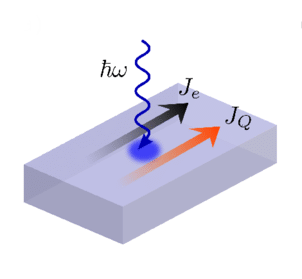
In this tutorial we will show how to calculate Shift Current in bulk materials.
We suppose you are already familiar with the non-linear response using the Yambo code.
If it is not the case please study the previous tutorials:
Linear response using Dynamical Berry Phase and Real time approach to non-linear response (SHG).
This theoretical implementation of this tutorial is described in the paper [1] , please cite it if you use it.
The tutorial was created with the help of Yuncheng Mao.
Setup calculations
In this tutorial we will take as example the two dimensional GeS monolayer.
DFT inputs can be downloaded here: GeS_DFT.tgz.
First of all run the setup, then remove symmetries along the y direction, as explained in the tutorial above.
Real-time setup and calculations
In order to generate input file for shift current you do: yambo_nl -u n -V par -F input.in
nloptics                         # [R] Non-linear spectroscopy
NLogCPUs=0                       # [PARALLEL] Live-timing CPU`s (0 for all)
PAR_def_mode= "balanced"         # [PARALLEL] Default distribution mode ("balanced"/"memory"/"workload"/"KQmemory")
NL_CPU= "8 1"                       # [PARALLEL] CPUs for each role
NL_ROLEs= "w k"                     # [PARALLEL] CPUs roles (w,k)
DIP_CPU= ""                      # [PARALLEL] CPUs for each role
DIP_ROLEs= ""                    # [PARALLEL] CPUs roles (k,c,v)
OSCLL_CPU= ""                    # [PARALLEL] CPUs for each role
OSCLL_ROLEs= ""                  # [PARALLEL] CPUs roles (k,b)
DIP_Threads=0                    # [OPENMP/X] Number of threads for dipoles
NL_Threads=0                     # [OPENMP/NL] Number of threads for nl-optics
OSCLL_Threads=0                  # [OPENMP/X] Number of threads for Oscillators
% NLBands
  17 |  24 |                           # [NL] Bands range
%
NLverbosity= "high"              # [NL] Verbosity level (low | high)
NLtime=-1.000000           fs    # [NL] Simulation Time
NLintegrator= "INVINT"           # [NL] Integrator ("EULEREXP/RK2/RK4/RK2EXP/HEUN/INVINT/CRANKNIC")
NLCorrelation= "IPA"             # [NL] Correlation ("IPA/HARTREE/TDDFT/LRC/LRW/JGM/SEX/LSEX/LHF")
NLLrcAlpha= 0.000000             # [NL] Long Range Correction
% NLEnRange
 1.000000 | 8.000000  |         eV    # [NL] Energy range (for loop on frequencies NLEnSteps/=0
%
NLEnSteps=  24                    # [NL] Energy steps for the loop on frequencies
% NLrotaxis
 0.000000 | 0.000000 | 0.000000 |        # [NL] Rotation axis (for the loop on angles NLAngSteps/=0)
%
NLAngSteps=0                     # [NL] Angular steps (if NLAngSteps/=0 field versor will be ignored)
NLDamping= 0.200000        eV    # [NL] Damping (or dephasing)
RADLifeTime=-1.000000      fs    # [RT] Radiative life-time (if negative RADLifeTime=Phase_LifeTime)
EvalCurrent                    # [NL] Evaluate the current
#FrPolPerdic                   # [DIP] Force periodicity of polarization respect to the external field
% Field1_Freq
 0.100000 | 0.100000 |         eV    # [RT Field1] Frequency
%
Field1_NFreqs= 1                 # [RT Field1] Frequency
Field1_Int=  1000.00       kWLm2 # [RT Field1] Intensity
Field1_Width= 0.000000     fs    # [RT Field1] Width
Field1_kind= "SOFTSIN"           # [RT Field1] Kind(SIN|SOFTSIN| see more on src/modules/mod_fields.F)
Field1_pol= "linear"             # [RT Field1] Pol(linear|circular)
% Field1_Dir
 0.000000 | 1.000000 | 0.000000 |        # [RT Field1] Versor
%
Field1_Tstart= 0.010000    fs    # [RT Field1] Initial Time
Notice that in this input we turned one the evaluation of current EvalCurrent and force the parallelization on the frequencies, NL_CPU= "8 1", NL_ROLEs= "w k", that is much more efficient than the one on k-points.
Then you can run simulation by doing: yambo_nl -F input.in
Analysis of the results
In order to analyze the result we use Yambopy: YamboPy,
and the following script for the post-processing:
from yambopy import *
from yambopy.nl.harmonic_analysis import Harmonic_Analysis
from yambopy.units import fs2aut
X_order=4
NLDB=YamboNLDB()
Harmonic_Analysis(NLDB,X_order=X_order,prn_Peff=True)
This script will produce different file containing the response function of the current and polarization respect to the total field.
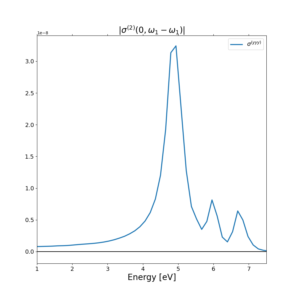
From the second order response of the current at zero frequency, file o.YamboPy-Sigma_probe_order_0 we can extract the shift current coefficient along the 'y' direction
that correspond to the 5th column of the file.
Hereafter we report the shift current spectrum compared with the results of Ibañez-Azpiroz et al. [2].
The python script to plot the results, the data from the Ibañez-Azpiroz paper can be downloaded here: GeS_plot.
In this example we used very few k-points, increasing the number of k-points bring the result very close to the one of Ibañez-Azpiroz, see also Supp. Mat. of Ref. [1] .
Notice that we rescale the shift-currect for an effective thickness of 2.65 Angstrom, you can find all the rescaling factor in the python script.
Correlation effects can be included in the SC response in the same way we do for other non-linear response functions, for more info look at the tutorial: SHG within the TD-aGW level (also called TD-HSEX, TD-BSE)
References
- ↑ 1.0 1.1 Yuncheng Mao, Myrta Grüning, Ju Zhou, and Claudio Attaccalite, Shift current in 2D Janus Transition-Metal Dichalcogenides: the role of excitons , arXiv: (2025)
- ↑ Julen Ibañez-Azpiroz, Stepan S. Tsirkin, and Ivo Souza, Ab initio calculation of the shift photocurrent by Wannier interpolation, Phys. Rev. B 107, 205204 (2023)

