Bethe-Salpeter on top of quasiparticle energies

In this module you will learn how to include GW-corrected (QP) energies in the calculation of the absorption spectrum. In order to do this, you need to have completed the tutorial on the BSE kernel and optionally already computed the absorption spectrum without QP corrections.

Reading the QP corrections from a previous GW calculation

In the above calculation we have used a simple scissor operator to correct the Kohn-Sam DFT energies. In this part we see how we can instead take the corrections from a previous Yambo Gw calculation. We create and edit the input:

$yambo -F 03_3D_QP_BSE.in -y d -V qp -J 3D_BSE

We set all parameters as in the previous calculation, except for the part regarding the QP correction:

 KfnQPdb= "E < 3D_QP_BSE/ndb.QP"              # [EXTQP BSK BSS] Database
 KfnQP_N= 1                   # [EXTQP BSK BSS] Interpolation neighbours
 % KfnQP_E
  0.000000 | 1.000000 | 1.000000 |        # [EXTQP BSK BSS] E parameters  (c/v) eV|adim|adim
%

Instead of setting the values for the scissor, we give the path to a database (3D_QP_BSE/ndb.QP) which contains the QP corrections. This has been created by running a GW calculation as in the GW tutorial. Run Yambo:

$ yambo -F 03_3D_QP_BSE.in -J "3D_QP_BSE,3D_BSE"

This produces the following log in the standard output. Note Section 4 (regarding external QP corrections to the kernel):

<01s> [04.01] External QP corrections (K)
<01s> [QP@K] E<3D_QP_BSE/ndb.QP[ PPA XG:39 Xb:1   40 Scb:1   40]
<01s> [QP] Kpts covered exactly  [o/o]: 100.0000

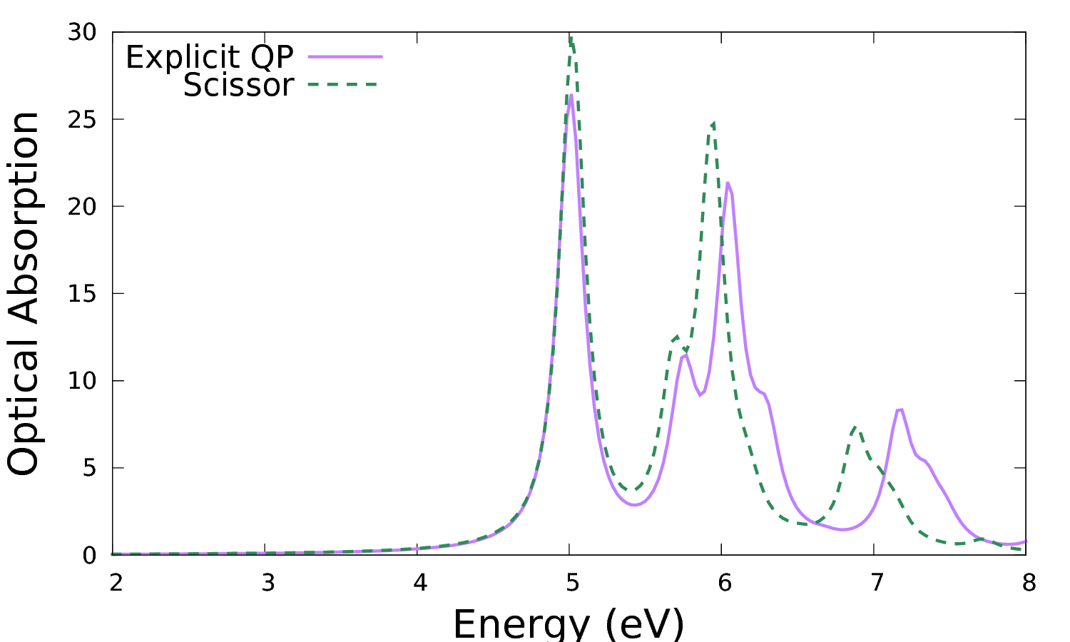
This tells you that the file was found, read correctly and that the k points found in the file matched the ones you are using for the current calculation (otherwise interpolation would be needed). It is crucial to check that the file has been read, since if not Yambo gives a warning but continues the calculation (with no QP corrections at all!). As in the previous calculation the final results of the calculation are the files with the spectral functions. Let's compare the results for the optical absorption spectrum with those obtained previously with a simple scissor:

$ gnuplot
...
plot 'o-3D_QP_BSE.eps_q1_diago_bse' u 1:2 w l t 'Explicit QP', 'o-3D_BSE.eps_q1_diago_bse' u 1:2 w l t 'Scissor' 

It is clear that this makes a difference in the peak distribution and intensity. Note that beside a simple shift you can renormalise as well the bandwidth of the valence and conduction bands in KfnQP_E (respectively the third and second value). You can try as an exercise to set up a new calculation using e.g. 1.440000 | 1.200000 | 0.900000 | for KfnQP_E.