Introduction to Real Time propagation in Yambo
Introduction
A new feature in yambo is the numerical integration of a time-dependent (TD) equation of motion (EOM), able to describe the evolution of the electronic system under the action of an external laser pulse. Similarly to the equilibrium case, the most diffuse ab initio approaches to real-time propagation are based on TD-DFT and there exist a number of GPL codes available to this end. On the contrary the implementation of real time propagation within MBPT is an almost unique feature of the yambo code. Two different schemes are available. In one case, the density matrix of the system, is propagated in time, as described in the first section. In the second case an effective time dependent Schrodinger equation for the occupied orbitals is propagated, as described in the second section.
Time Dependent Equation for the Reduced One--Body Density--Matrix
The first scheme is a Time Dependent equation for the one body reduced density matrix. The EOM for the density matrix projected in the space of the single particle wave-functions is derived from non-equilibrium (NEQ) many-body perturbation theory and reads
Here we underline quantities which are vectors in the transition space. The Hamiltonian contains the equilibrium eigenvalues plus the variation of the self-energy.
![]() represents the external potential written in the length gauge; shape, polarization, intensity (and eventually frequency) of the field E can be selected in input. r is the position operator. The coupling to the external field is exact up to first order.
represents the external potential written in the length gauge; shape, polarization, intensity (and eventually frequency) of the field E can be selected in input. r is the position operator. The coupling to the external field is exact up to first order.
Linear Response
From the knowledge of the density matrix, the first order polarization
![]() is computed at each time step. The spectrum of the system can then be obtained by the Fourier transform of the polarization,
which can be done as a post-processing step. Absorption is thus obtained via the dipole-dipole response function (equivalent
to the length gauge in linear response).
[math]\displaystyle{ \chi(\omega) = \frac{P(\omega)}{E(\omega)} }[/math]
is computed at each time step. The spectrum of the system can then be obtained by the Fourier transform of the polarization,
which can be done as a post-processing step. Absorption is thus obtained via the dipole-dipole response function (equivalent
to the length gauge in linear response).
[math]\displaystyle{ \chi(\omega) = \frac{P(\omega)}{E(\omega)} }[/math]
More details will be given during the tutorials:
Time Dependent Effective Schrödinger Equation
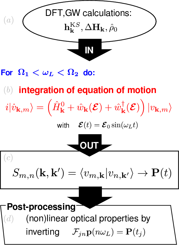
The second scheme is a Time Dependent Effective Schrödinger Equation(TD-ESE), where the coupling between electrons and the external field is described by means of the Modern Theory of Polarization:
Where [math]\displaystyle{ | v_{i \mathbf{k}} \rangle }[/math] are the time-dependent valence bands, Hsysk is the Hamiltonian, [math]\displaystyle{ \mathcal E(t) }[/math] is the external field and the term [math]\displaystyle{ i e \partial k }[/math] corresponds to the dipole operator in periodic systems. For more details on this last term see Ref. [1] and [2].
Differently from other codes, the equations of motion of Yambo are in the length gauge and not in the velocity one. If you want to know more about the advantages and disadvantages of the two gauges read section 2.7 of Ref. [3].
The Hamiltonian and the initial wave-functions are obtained from DFT. Then in order to obtain linear response, we probe the system with a delta function field, that excites all the frequencies at the same footing, and Fourier transforms. We calculate the Berry polarization
Linear Response
In general the induced polarization is the sum of the responses of the system to all orders in the external field: [math]\displaystyle{ \bf{P}(t) = \sum_{n=-\infty}^{+\infty} \bf{P}_n (t) }[/math] If the perturbation is weak enought the response is dominated by the first order term and from its Fourier transform we get the response function. Indeed
[math]\displaystyle{ \chi(\omega) = \frac{P(\omega)}{E(\omega)} }[/math]
that is related to the dielectric constant through the relation [math]\displaystyle{ \epsilon(\omega) = 1 + 4 \pi \chi(\omega) }[/math]. See also Ref. [2]
More details will be given during the tutorials:
Non Linear Response
Non-linear response calculations are similar to the linear response case, with the only difference that we excite the system with a sinusoidal external field. A perturbation with a specific frequency allows to expand the polarization in the form [math]\displaystyle{ \bf{P}(t) = \sum_{n=-\infty}^{+\infty} \bf{p}_n e^{-i\omega_n t} }[/math] where the coefficient [math]\displaystyle{ \bf{p}_1,...,\bf{p}_n }[/math] are related to [math]\displaystyle{ \chi^{(1)},...,\chi^{(n)} }[/math]. In practice we use the scheme described in Ref. [4] and show below to extract the non-linear coefficients:
More details will be given during the tutorials:
References
- ↑ I. Souza, J. Íñiguez, and D. Vanderbilt, PRB 69, 085106 (2004)
- ↑ 2.0 2.1 C. Attaccalite and M. Gruning Rev. B, 88, 235113 (2013)
- ↑ C. Attaccalite, arXiv 1609.09639 (2017)
- ↑ C. Attaccalite and M. Gruning, Rev. B, 88, 235113 (2013)


