How to choose the input parameters

In the previous tutorial, you have been guided step-by-step through the calculations of the optical spectrum of bulk hBN by solving the Bethe-Salpeter equation. The values for the relevant input parameters have then been given to you.

In this tutorial you will learn how to choose those parameters. These parameters are related either to the truncation of infinite sums or to the approximations of infinitesimal with small, but finite quantities. A wrong choice of these parameters can lead to inaccurate or even physically wrong results. One then needs to run a series of calculations by changing the parameters till the results are converged , meaning they are changing by a negligible amount.

Note that all the following operations can be automated. A useful python-based interface to yambo, yambopy, can be used for this purpose. It is worth however to go at least once through the pain of a 'by-hand' convergence study so to better understand the automated process for few of those variables.

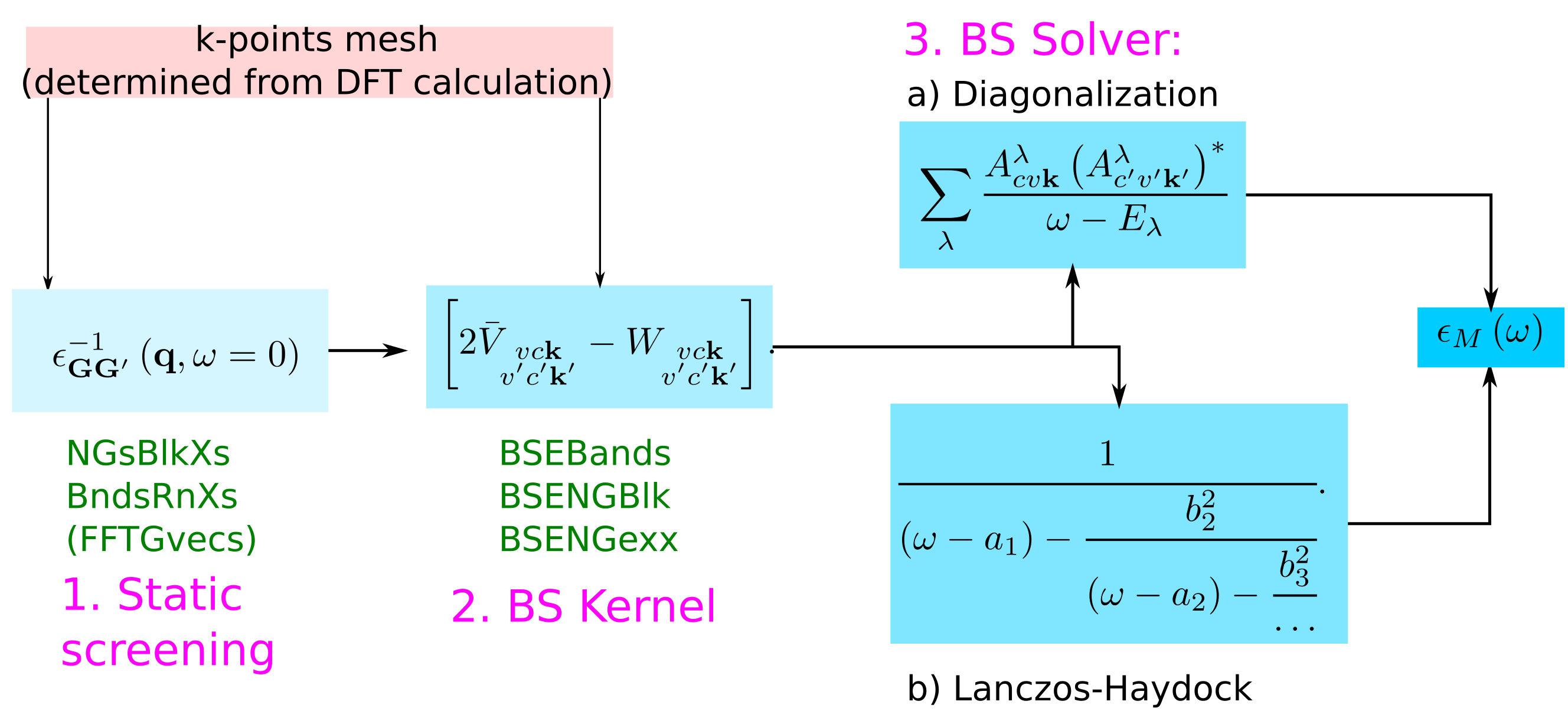
Coming back to the scheme to calculate the macroscopic dielectric matrix within Bethe-Salpeter, here the list of the parameters that have to be determined by convergence studies:

Though we will discuss those parameters, we will run examples only for the BS kernel part.

Convergence of the static screening

The parameters that need to be converged can be understood by looking at the equations:

where χ_GG' is given by

• NGsBlkXs : The dimension of the microscopic inverse matrix, related to Local fields
• BndsRnXs : The sum on bands in the independent particle χ⁰_GG'

Furthermore as shown in this tutorial one can reduce the value of

• FFTGvecs

since generally, fewer G-vectors are needed than what are needed in DFT calculations. This can be critical for large calculations, or for supercells with a lot of vacuum. Note that this parameter appear only when the input is generated specifying the verbosity level -V RL

The convergence for the static screening then is similar to the convergence of other response functions and the plasmon pole in GW calculations and won't be covered here. Note in fact that you can re-use the database obtained (and converged) from a previous plasmon pole calculation as long as the same k-points are used

ADD COMMAND

Convergence of the macroscopic dielectric function

In the expression for the macroscopic dielectric function

depends on the summation over the pair of quasiparticle states vck.

• BSEBands : defines the vc pairs.
• the k-point mesh of the DFT calculations defines the k

Basically we need a large enough basis of transitions (pair of quasiparticle states) to correctly describe the excitons in the energy region of interest.

Furthermore, in the kernel part

summations over G vectors appear:

• BSENGblk: defines the screened interaction block size (double sum in W).
• BSENGexx: defines the components of Hartree potential (the sum in V).

In the following we will see how the spectrum depends on these parameters.

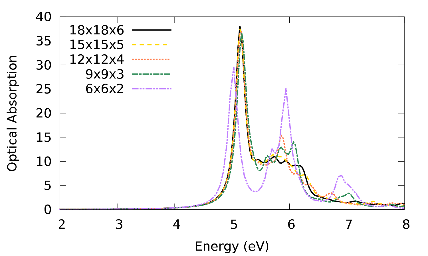
Convergence with the k-point mesh

For this part you need the SAVE databases for different meshes which are contained in the corresponding folders:

9x9x3 12x12x4 15x15x5 18x18x6

Following the scheme we learned in previous tutorial:

- Enter the 9x9x3 directory - Run the initialization - Create the input for calculating the screening:

 $ yambo -F 02_screening.in -J 3D_993 -b

- Modify the input as follows

NGsBlkXs = 4 Ry
%BndsRnXs
1 | 40 |
%
%LongDrXS
1.000 | 1.000 | 1.000|
%

- Run the calculation for the screening

$ yambo -F 02_screening.in -J 3D_993

- Create the input for calculating the macroscopic dielectric function:

$ yambo -F 03_bse.in -J 3D_993 -o b -k sex -y h -V qp

Which combines the BS kernel + BS solver (Lanczos-Haydock) runlevels - Modify the input as follows

BSENGexx = 30 Ry
BSENGBlk = 4 Ry
% BSEBands
 6 | 10 |       
%
% BEnRange
  2.00000 | 8.00000 | eV    
%
BEnSteps= 200      
% BDmRange
  0.10000 |  0.10000 | eV    
%
% BLongDir
 1.000000 | 1.000000 | 0.000000 | 
%
% KfnQP_E 
 1.440000 | 1.000000 | 1.000000 |
%
BSHayTrs= 0.02000

- Launch the calculation:

$ yambo -F 03_bse.in -J 3D_993

-Repeat the procedure for the 12x12x4 with the difference you will use a different prefix: -J 3D_12124.

The convergence on the k-point is the most expensive part. Note that for the two larger meshes the calculations of both the screening and kernel take several minutes. If short of time postpone these calculations. If you have the time and computational resources repeat the above procedure for 15x15x5 and 18x18x6. Note that the BS kernel starts becoming very (too) large and you need to fragment it to speed up the IO. Then after generating and modifying the input the input invoke yambo again as:

$ yambo -F 03_bse.in -J 3D_15155 -o b -k sex -y h -V io

and modify the variable

 DBsFRAGpm= "+BS"

After that launch the calculation

$ yambo -F 03_bse.in -J 3D_15155

If you correctly followed the above procedure you have a file of the optical absorption spectrum for each mesh, e.g. o-3D_18186.eps_q1_haydock_bse. To see at the effect of k-points plot those files with gnuplot:

$ gnuplot
> plot '18x18x6/o-3D_18186.eps_q1_haydock_bse' w l t '18x18x6, '15x15x5/o-3D_15155.eps_q1_haydock_bse' w l t '15x15x5', . . .
  . . . '12x12x4/o-3D_12124.eps_q1_haydock_bse' w l t '12x12x4, '9x9x3/o-3D_993.eps_q1_haydock_bse' w l t '9x9x3', '6x6x2/o-3D_662.eps_q1_haydock_bse' w l t '6x6x2'