Sum frequency generation
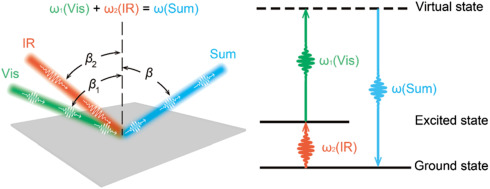
In this tutorial we will show how to calculate Sum Frequency Generation(SFG) and also Difference Frequency Generation (DFG) in bulk materials.
We suppose you are already familiar with the non-linear response using the Yambo code.
If it is not the case please study the previous tutorials:
Linear response using Dynamical Berry Phase and Real time approach to non-linear response (SHG).
We thank Mike N. Pionteck for the script used in this tutorial.
DFT calculations
In this example, we will consider a single layer of hexagonal boron nitride (hBN). If you didn't before you can download input files and Yambo databases for this tutorial here: hBN-2D-RT.tar.gz. and/or follow the instructions to generate the databases here: Prerequisites for Real Time propagation with Yambo
Removing symmetries
In this tutorial we will calculate the SFG along when both fields are in the 'y' direction,
therefore we remove symmetries not compatible with an external field along this direction, with the command ypp_nl -y:
fixsyms                          # [R] Remove symmetries not consistent with an
external perturbation
% Efield1
  0.000000 | 1.000000 | 0.000000 |        # First external Electric Field
%
% Efield2
 0.000000 | 0.000000 | 0.000000 |        # Additional external Electric Field
%
BField= 0.000000           T     # [MAG] Magnetic field modulus
Bpsi= 0.000000             deg   # [MAG] Magnetic field psi angle [degree]
Btheta= 0.000000           deg   # [MAG] Magnetic field theta angle [degree]
#RmAllSymm                     # Remove all symmetries
RmTimeRev                     # Remove Time Reversal
#RmSpaceInv                    # Remove Spatial Inversion
Real-time simulation with two external fields
You go in the FixSymm folder and run again the setup. Then you can put the following input file, that has been generated with the command yambo_nl -u n , in the folder with the name yambo.in_sfg:
nloptics                         # [R] Non-linear spectroscopy
NLogCPUs=0                       # [PARALLEL] Live-timing CPU`s (0 for all)
PAR_def_mode= "balanced"         # [PARALLEL] Default distribution mode ("balanced"/"memory"/"workload"/"KQmemory")
NL_CPU= "10 1"                       # [PARALLEL] CPUs for each role
NL_ROLEs= "w k"                     # [PARALLEL] CPUs roles (w,k)
DIP_CPU= ""                      # [PARALLEL] CPUs for each role
DIP_ROLEs= ""                    # [PARALLEL] CPUs roles (k,c,v)
DIP_Threads=0                    # [OPENMP/X] Number of threads for dipoles
NL_Threads=0                     # [OPENMP/NL] Number of threads for nl-optics
% NLBands
   3 |  6 |                           # [NL] Bands range
%
NLverbosity= "low"              # [NL] Verbosity level (low | high)
NLtime= 60.00000           fs    # [NL] Simulation Time
NLintegrator= "CRANKNIC"         # [NL] Integrator ("EULEREXP/RK2/RK4/RK2EXP/HEUN/INVINT/CRANKNIC")
NLCorrelation= "IPA"             # [NL] Correlation ("IPA/HARTREE/TDDFT/LRC/LRW/JGM/SEX")
NLLrcAlpha= 0.000000             # [NL] Long Range Correction
% NLEnRange
  2.000000 | 8.000000 |         eV    # [NL] Energy range (for loop on frequencies NLEnSteps/=0
%
 NLEnSteps= 30                  # [NL] Energy steps for the loop on frequencies
% NLrotaxis
 0.000000 | 0.000000 | 0.000000 |        # [NL] Rotation axis (for the loop on angles NLAngSteps/=0)
%
NLAngSteps=0                     # [NL] Angular steps (if NLAngSteps/=0 field versor will be ignored)
NLDamping= 0.200000        eV    # [NL] Damping (or dephasing)
RADLifeTime=-1.000000      fs    # [RT] Radiative life-time (if negative Yambo sets it equal to Phase_LifeTime in NL)
#EvalCurrent                   # [NL] Evaluate the current
#FrPolPerdic                   # [DIP] Force periodicity of polarization respect to the external field
HARRLvcs= 18475            RL    # [HA] Hartree     RL components
EXXRLvcs= 18475            RL    # [XX] Exchange    RL components
 % Field1_Freq
-0.100000 |-0.100000 |         eV    # [RT Field1] Frequency
%
Field1_NFreqs= 1                 # [RT Field1] Frequency
Field1_Int=   1000.00       kWLm2 # [RT Field1] Intensity
Field1_Width= 0.000000     fs    # [RT Field1] Width
Field1_kind= " SOFTSIN"           # [RT Field1] Kind(SIN|SOFTSIN| see more on src/modules/mod_fields.F)
Field1_pol= "linear"             # [RT Field1] Pol(linear|circular)
% Field1_Dir
  0.000000 | 1.000000 | 0.000000 |        # [RT Field1] Versor
%
Field1_Tstart= 0.010000    fs    # [RT Field1] Initial Time
% Field2_Freq
2.000000 | 2.000000 |         eV    # [RT Field2] Frequency
%
Field2_NFreqs= 1                 # [RT Field2] Frequency
Field2_Int=   1000.00       kWLm2 # [RT Field2] Intensity
Field2_Width= 0.000000     fs    # [RT Field2] Width
Field2_kind= " SOFTSIN"           # [RT Field2] Kind(SIN|SOFTSIN| see more on src/modules/mod_fields.F)
Field2_pol= "linear"             # [RT Field2] Pol(linear|circular)
% Field2_Dir
  0.000000 | 1.000000 | 0.000000 |        # [RT Field2] Versor
%
Field2_Tstart= 0.010000    fs    # [RT Field2] Initial Time
If you run this input file with the command yambo_nl -F yambo.in_sfg, the code will run 30 simulations for a first laser field with frequency between 2.0 and 8.0 while the frequency of the second field is fixed at 2.0 eV. For this reason we provide you a simple python script to change also the frequency of the second field (in blue in the input).
please modify the python script by set the correct path of your executable, the parallelization and the number of frequency steps you are interested in. In this example we will do 30 frequency steps for both the first (in the Yambo input) and the second field (in the python script).
Calculations will take some time, in the above example we parallelized on 10 cores to speed up them.
When the calculations are terminated you will find many folders called EF1, EF2, ... EF29. These folders are generated from the loop on the second field frequency(Field2_Freq), and each one contains the response real-time polarization at 30 different frequencies of the first external field (Field1_Freq).
Analysis of the results
Now we have to analyze the results, we will use an extension to two fields of the approach described in Ref. [1] and used for the tutorials on second/third harmonic generation: Real time approach to non-linear response (SHG). These new subroutine are available in the new YamboPy package. Hereafter the script to read all the real-time polarization, Fourier analize them and
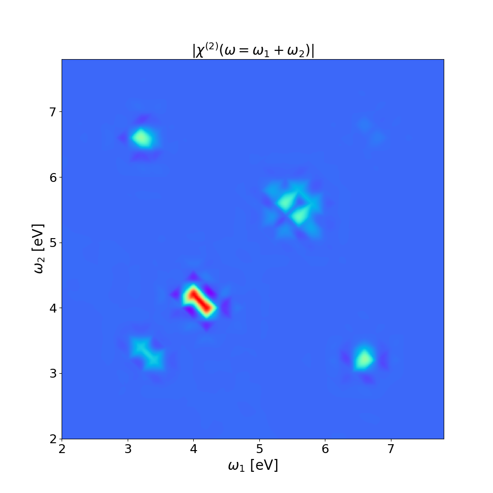
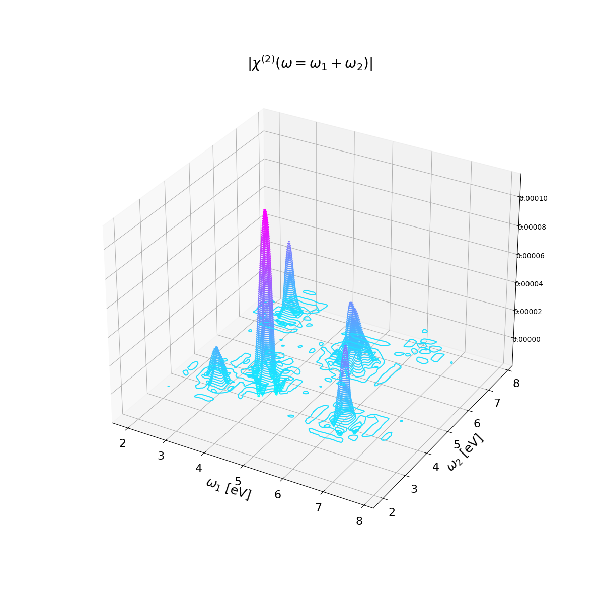
write the [math]\displaystyle{ \chi^{(2)}(\omega=\omega_1 + \omega_2) }[/math] in a file in the form: [math]\displaystyle{ \omega_1 , \omega_2, Re \{\chi^{(2)}\} , Im \{\chi^{(2)}\} }[/math].
Comparison with SHG
- ↑ Nonlinear optics from an ab initio approach by means of the dynamical Berry phase: Application to second- and third-harmonic generation in semiconductors, C. Attaccalite and M. Grüning, Phys. Rev. B 88, 235113(2013)


