Second-harmonic generation of 2D-hBN
Step 0: Theoretical framework
In this tutorial, we compute the Second-harmonic generation (SHG) from the dynamics of the Bloch-states. The equation-of-motion of the Bloch-states is explained in the tutorial on Linear response from Bloch-states dynamics. Independently of the 'experiment' we simulate, the part of the integration of motion stays the same. This means that any experiment, including non-linear optics, can be performed at the level of the theory listed for the computation of the dielectric function:
- independent (quasi)particle
- time-dependent Hartree (RPA level)
- time-dependent DFT (and DPFT)
- time-dependent Hartree+Screened exchange (BSE level)
What changes when we want to calculate the SHG (or higher harmonics) is:
- the time-dependence of the input electric field and
- the post-processing of the signal
Time dependence of the electric Field: we choose a sinusoidal electric field, thus a monochromatic laser field. This allows one to expand the polarization in the form [math]\displaystyle{ \bf{P}(t) = \sum_{n=-\infty}^{+\infty} \bf{p}_n e^{-i\omega_n t} }[/math] where the coefficient [math]\displaystyle{ \bf{p}_1,...,\bf{p}_n }[/math] are related to [math]\displaystyle{ \chi^{(1)},...,\chi^{(n)} }[/math] through a coefficient depending on a power of the strength of the field (with the power depending on the order of the response).
At difference with a delta-like perturbation, a real-time simulation gives the response at the laser-field only. Then, to obtain the spectrum for the desired range of frequency, we have to perform so many simulations as the frequencies in the desired range.
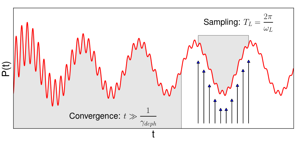
Post-processing of the signal: The switch-on of the electric field corresponds to a weak delta-like kick. Thus, even if it may not be noticeable, the polarization results from both the sinusoidal field and the delta-like kick. The latter excites all eigenfrequencies of the system. Though weak, the resulting signal is comparable with the second-harmonic signal. To eliminate the signal from the eigenfrequencies, we apply a dephasing ([math]\displaystyle{ \gamma_{deph} }[/math]). To have a signal useful to sample the second-harmonic signal, we need to wait a time [math]\displaystyle{ \bar t }[/math] much larger than the dephasing-time [math]\displaystyle{ 1/\gamma_{deph} }[/math]. Note that we cannot choose a too short dephasing time (to shorten the simulation time), as this would result in a too large broadening of the spectrum. After [math]\displaystyle{ \bar t }[/math], we sample 2N+1 times in a period and use discrete Fourier transform to extract [math]\displaystyle{ {p}_n }[/math] for [math]\displaystyle{ n = 0,...,N }[/math], where n=2 gives the SHG. This is schematically illustrated in figure:
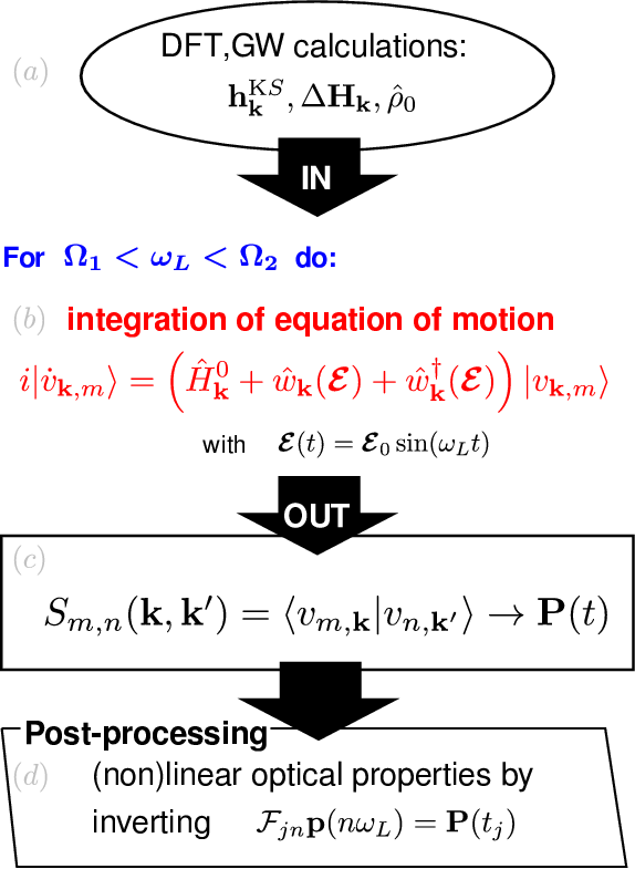
The scheme from Ref. [1] summarised the workflow for computing the SHG (or higher-harmonics) in a energy range [math]\displaystyle{ [\Omega_1,\Omega_2] }[/math].
Step 1: Prerequisites
You should be in the folder YAMBO_TUTORIALS/hBN-2D/YAMBO/.
In this example, we will consider a single layer of hexagonal boron nitride (hBN). Before running real time simulations to compute the SHG in yambo you need to download input files and Yambo databases for this tutorial here: wget https://media.yambo-code.eu/educational/tutorials/files/hBN-2D.tar.gz hBN-2D.tar.gz.
Unzip the tarball and change directory to YAMBO and run the setup (yambo_nl -nompi).
Execute the command
ypp_nl -fixsym -F 00_removesym.in
to create the input, to remove the symmetries which are not compatible with the field:
fixsyms                          # [R] Remove symmetries not consistent with an external perturbation
% Efield1
 1.000000 | 1.000000 | 0.000000 |        # First external Electric Field
%
% Efield2
 0.000000 | 0.000000 | 0.000000 |        # Additional external Electric Field
%
BField= 0.000000           T     # [MAG] Magnetic field modulus
Bpsi= 0.000000             deg   # [MAG] Magnetic field psi angle [degree]
Btheta= 0.000000           deg   # [MAG] Magnetic field theta angle [degree]
#RmAllSymm                     # Remove all symmetries
RmTimeRev                     # Remove Time Reversal
#RmSpaceInv                    # Remove Spatial Inversion
#KeepKGrid                     # Do not expand the k-grid
where we chose the field along the xy direction and we remove time-reversal symmetry.
Then run the pre-processing job:
ypp_nl -F 00_removesym.in J 00_removesym
This creates the directory FixSymm. Change directory to FixSymm. This contains the SAVE directory with reduced symmetries, compatible with the direction of the field. Now run the setup again (yambo_nl -nompi).
Step 2: Independent-particle approximation
Use the command:
yambo_nl -nl n -F 01_SHG_ip.in
to generate the input:
nloptics                         # [R] Non-linear spectroscopy
% NLBands
   3 |  6 |                         # [NL] Bands range
%
NLverbosity= "high"              # [NL] Verbosity level (low | high)
NLtime=-1.000000           fs    # [NL] Simulation Time
NLintegrator= "INVINT"           # [NL] Integrator ("EULEREXP/RK2/RK4/RK2EXP/HEUN/INVINT/CRANKNIC")
NLCorrelation= "IPA"             # [NL] Correlation ("IPA/HARTREE/TDDFT/LRC/LRW/JGM/SEX")
NLLrcAlpha= 0.000000             # [NL] Long Range Correction
% NLEnRange
 0.5000000 |8.000000 |         eV    # [NL] Energy range
%
NLEnSteps= 12                     # [NL] Energy steps
NLDamping= 0.200000        eV    # [NL] Damping (or dephasing)
RADLifeTime=-1.000000      fs    # [RT] Radiative life-time (if negative Yambo sets it equal to Phase_LifeTime in NL)
#EvalCurrent                   # [NL] Evaluate the current
#FrPolPerdic                   # [DIP] Force periodicity of polarization respect to the external field
HARRLvcs= 1000            mHa   # [HA] Hartree     RL components
EXXRLvcs= 1000            mHa    # [XX] Exchange    RL components
% Field1_Freq
0.100000 | 0.100000 |         eV    # [RT Field1] Frequency
%
Field1_NFreqs= 1                 # [RT Field1] Frequency
Field1_Int=  1000.00       kWLm2 # [RT Field1] Intensity
Field1_Width= 0.000000     fs    # [RT Field1] Width
Field1_kind= "SIN"           # [RT Field1] Kind(SIN|COS|RES|ANTIRES|GAUSS|DELTA|QSSIN)
Field1_pol= "linear"             # [RT Field1] Pol(linear|circular)
% Field1_Dir
 1.000000 | 1.000000 | 0.000000 |        # [RT Field1] Versor
%
Field1_Tstart= 0.010000    fs    # [RT Field1] Initial Time
To describe the Bloch-dynamics we will use as a basis the KS-states 3-6 for the k-grid used in the non-scf DFT calculations, that is a 6x6x1 (NLBands). We choose 12 equally spaced frequencies (NLEnSteps) for the applied field in the range (NLEnRange) between 0.5 and 8 eV. We choose a sinusoidal time-dependence (Field1_kind) and set the field direction (Field1_kind) along xy (in plane). The negative simulation time (NLtime=-1.000000) means that the code will choose it based on the value of the NLDamping. While this is a good lower bound for the simulation time, one should check it is sufficient to get accurate results.
Run the simulation, possibly in parallel e. g. in a interactive session on 4 cores.
[In order to get 4 cores while in an interacting node, exit your current allocation and rerun salloc asking for the proper number of tasks:
salloc -A tra23_Yambo -p m100_usr_prod -q m100_qos_dbg --nodes=1 --ntasks-per-node=4 --cpus-per-task=4 -t 02:00:00
Otherwise, you can submit the job with a slurm script as explained in the introductory page]
Now execute the command:
mpirun -n 4 yambo_nl -F 01_SHG_ip.in -J 01_SHG_ip -C 01_SHG_ip_files
This run will take several minutes. While it is running, you can check the progress of one specific frequency:
tail -f 01_SHG_ip_files/o-01_SHG_ip.polarization_F2
If you want to know how many fs the simulation will last (since this was decided by the code), you can get this information in the report file:
$ grep Total 01_SHG_ip_files/r-01_SHG_ip_nloptics
Total simulation time       :  41.23193 [fs]
If you instead want to track the progress of the full simulation, you should check the log file(s). If you are doing a parallel run, you can type
tail -f 01_SHG_ip_files/LOG/l-01_SHG_ip_nloptics_CPU_1
Once the run is finished, check the report 01_SHG_ip_files/r-01_SHG_ip_nloptics. In particular, in the appended input files, you can see the default parallelization applied by the code for calculating the dipoles and run the time-propagation. For the latter, the main parallelization is on the frequencies and then on the k-points (NL_ROLEs= "w.k").
| NL_CPU= "2.2"                    # [PARALLEL] CPUs for each role
| NL_ROLEs= "w.k"                  # [PARALLEL] CPUs roles (w,k)
| DIP_CPU= "2.2.1"                 # [PARALLEL] CPUs for each role
| DIP_ROLEs= "v.c.k"               # [PARALLEL] CPUs roles (k,c,v)
Also, look at the simulation time. This is approximately 42 fs.
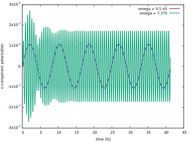
Plot the polarization for a couple of frequencies, e.g. the first and last of the chosen range (the corresponding frequency can be read in the file, search for "Frequency value"):
set ylabel "x-component polarization" offset -0.7
set xlabel "time (fs)"
plot '01_SHG_ip_files/o-01_SHG_ip.polarization_F1' u 1:2 w l lw 2 title "omega = 0.5 eV"
replot '01_SHG_ip_files/o-01_SHG_ip.polarization_F12' u 1:2 w l lw 2  title "omega = 7.375 eV"
After the applied field is 'switched on', the polarization is oscillating at the frequency of the applied field and at the eigenfrequencies of the system as described above in the cartoon. This is visible particularly for the higher frequency. Due to the dephasing, after about 20 fs the polarization is oscillating (at least to the eye) at the frequency of the applied field. Nonlinear components are not visible since they are several orders of magnitude smaller than the first order.
Output post-processing: the dielectric function
Once we obtained the polarization, we Fourier-transform the polarization to obtain the dielectric function.
Use the command:
ypp_nl -nl -F 02_SHG_ip_pp.in -C 01_SHG_ip_files
to generate the input file:
nonlinear                        # [R] Non-linear response analysis
<span style="color:red"Xorder= 4 # Max order of the response/exc functions
% TimeRange
 -1.000000 |-1.000000 |         fs    # Time-window where processing is done
%
ETStpsRt= 200                    # Total Energy steps
% EnRngeRt
  0.00000 | 20.00000 |         eV    # Energy range
%
DampMode= "NONE"                 # Damping type ( NONE | LORENTZIAN | GAUSSIAN )
DampFactor= 0.000000       eV    # Damping parameter
PumpPATH= "none"                 # Path of the simulation with the Pump only
Where we changed the Xorder to 4. This variable controls the terms in the Fourier expansion of the polarization. We choose up to expand up to the fourth order. This should ensure the second order to be accurate enough. As an exercise, you can change this value (e.g. choose 2,3,5,6) and see how the result below is changing. The time-window where processing is done is chosen automatically, since values are negative. The code chooses by default the last period to carry out the analysis.
To run the post-processing, use the command:
ypp_nl -F Inputs_shg/ypp_shg.in -J TD-IP_nl -C TD-IP_nl.
In 01_SHG_ip_files the following files were generated
o-01_SHG_ip.YPP-X_probe_order_1
o-01_SHG_ip.YPP-X_probe_order_2
o-01_SHG_ip.YPP-X_probe_order_3
o-01_SHG_ip.YPP-X_probe_order_4
r-01_SHG_ip_nonlinear
The output files contain respectively the first, second, third and fourth order response(corresponding to Xorder=4) at the 12 frequencies in the chosen range.
Inspect o-01_SHG_ip.YPP-X_probe_order_2
#     E [eV]            X/Im[cm/stV](x)    X/Re[cm/stV](x)    X/Im[cm/stV](y)    X/Re[cm/stV](y)    X/Im[cm/stV](z)    X/Re[cm/stV](z)
#
     0.50000000        -0.35378838E-09    -0.19774796E-07     0.23591828E-09    -0.89405637E-09      0.0000000          0.0000000
     1.1250000         -0.19356524E-08    -0.23160605E-07    -0.16052184E-09    -0.67662771E-09      0.0000000          0.0000000
     1.7500000         -0.69446459E-08    -0.35586956E-07    -0.76025706E-09    -0.10205678E-08      0.0000000          0.0000000
     2.37500000        -0.181606152E-7    -0.261823658E-8     0.438358596E-8     0.407915226E-8      0.00000000         0.00000000
The first column are the frequencies of the applied field, the second and third is the polarization along x (imaginary and real part), the fourth and fifth is the polarization along y (imaginary and real part) and the sixth and seventh is the polarization along z (imaginary and real part).
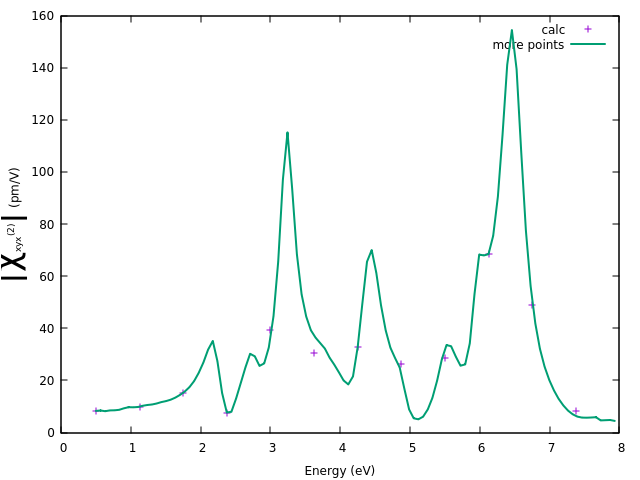
Plot the absolute value of the SHG for the "xxy" component (that is, the applied field is in the x and y directions and one look at the polarization along x):
set ylabel "{/Symbol=26 \174}{/Symbol=26 c}_{xyx}^{(2)}{/Symbol=26 \174} (pm/V)" offset -0.7
set xlabel "Energy (eV)"
pmVm1toCGS=2.38721e-09
plot '01_SHG_ip_files/o-01_SHG_ip.YPP-X_probe_order_2' u 1:(sqrt($2**2+$3**2)/pmVm1toCGS) w p title "calc"
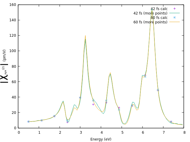
In the figure above, the results of the current run are compared with those for a run with 112 frequencies (one can obtain these results by repeating the calculations, changing the number of frequencies in NLEnSteps though this take about 10 times more computational time than the run with 12). One can notice some differences between the two runs. In fact, the two runs evaluate different frequnecies and the difference indicates spurious oscillations of the value of the polarizability due to the simulation time being too short and thus to the presence of 'noise' due to the eigenfrecies.
As an exercise, you can repeat the simulation for e,g, a time of 60 fs, that is setting NLtime=60. The plot below compare the SHG extracted at 42 fs and 60 fs, where the latter gives clearly more accurate results.
As a final note, the SHG depends on the size of the vacuum added in the supercell. Instead, one should consider the surface SHG which obtained by considering an effective thickness for the layer. This is usually chosen to be similar to the layer separation in the bulk counterpart.
Step 3: Hartree+Screened exchange approximation (BSE level)
Hartree+Screened exchange collisions
Similarly to the linear part, one needs to generate the Screened exchange collisions. The procedure is exactly the same.
Create the input:
yambo_nl -X s -e -v hsex -F 03_coll_hsex.in
modify the input ad follows
em1s                             # [R][Xs] Statically Screened Interaction
collisions                       # [R] Collisions
dipoles                          # [R] Oscillator strenghts (or dipoles)
Chimod= "HARTREE"                # [X] IP/Hartree/ALDA/LRC/PF/BSfxc
% BndsRnXs
   1 |  20 |                         # [Xs] Polarization function bands
%
NGsBlkXs= 1000 mHa    # [Xs] Response block size
% LongDrXs
 1.000000 | 1.000000 | 0.000000 |        # [Xs] [cc] Electric Field
%
% COLLBands
   4 |  5 |                         # [COLL] Bands for the collisions
%
HXC_Potential= "SEX+HARTREE"     # [SC] SC HXC Potential
HARRLvcs= 1000 mHa    # [HA] Hartree     RL components
EXXRLvcs= 1000 mHa    # [XX] Exchange    RL components
CORRLvcs= 1000 mHa    # [GW] Correlation RL components
Calculate the collisions (you may want to run in parallel):
yambo_nl -F 03_coll_hsex.in -J 03_coll -C 04_hsex_files
Run the simulation
Create the input:
yambo_nl -nl n -v hsex -V qp -F 04_SHG_hsex.in
modify the following parts of the input (by this time all the innput variables should be known from the previous exercises):
% BndsRnXs
  1 |  20 |                         # [Xs] Polarization function bands
%
NGsBlkXs= 1000 mHa    # [Xs] Response block size
% LongDrXs
 1.000000 | 1.000000 | 0.000000 |        # [Xs] [cc] Electric Field
%
% NLBands
   4 |  5 |                         # [NL] Bands range
%
NLintegrator= "CRANKNIC"           # [NL] Integrator ("EULEREXP/RK2/RK4/RK2EXP/HEUN/INVINT/CRANKNIC")
NLCorrelation= "SEX"             # [NL] Correlation ("IPA/HARTREE/TDDFT/LRC/LRW/JGM/SEX")
% NLEnRange
 0.500000 |8.000000 |         eV    # [NL] Energy range
%
NLEnSteps= 12                   # [NL] Energy steps
% GfnQP_E
 3.000000 | 1.000000 | 1.000000 |        # [EXTQP G] E parameters  (c/v) eV|adim|adim
%
Field1_kind= "SIN" # [RT Field1] Kind(SIN|COS|RES|ANTIRES|GAUSS|DELTA|QSSIN)
% Field1_Dir
 1.000000 | 1.000000 | 0.000000 |        # [RT Field1] Versor
%
Then run the simulation using e.g. mpi and 4 cores:
mpirun -n 4 yambo_nl -F 04_SHG_hsex.in -J 04_SHG_hsex,03_coll -C 04_SHG_hsex_files
Postprocessing: obtain the nonlinear response
Similarly to what we did for the independent particle case, we create the input:
ypp_nl -nl -F 05_SHG_hsex_pp.in
we change Xorder = 4 and then run:
ypp_nl -F 05_SHG_hsex_pp.in -J 04_SHG_hsex -C 04_hsex_files
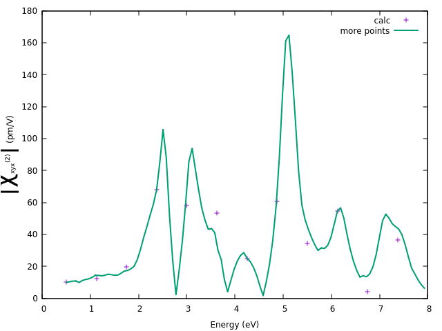
Then we plot (as before we compare with a simulation ran for 112 frequencies).
Plot the results:
set ylabel "{/Symbol=26 \174}{/Symbol=26 c}_{xyx}^{(2)}{/Symbol=26 \174} (pm/V)" offset -0.7
set xlabel "Energy (eV)"
pmVm1toCGS=2.38721e-09
plot '04_hsex_files/o-04_SHG_hsex.YPP-X_probe_order_2' u 1:(sqrt($2**2+$3**2)/pmVm1toCGS) w p title "calc"
Also in this case, we note differences between the two simulations. As discussed for the independent particle approximation, this is due to the too short simulation time. Repeating the calculations with a longer time gives more accurate results. In addition, note that in the interest of time, all parameters are under converged. In principle, to calculate the collisions one should use the same parameters of a converged BSE calculation. As well, to eliminate spurious interaction with the periodic images, one should use the Coulomb cut-off as it was used for this system in the tutorial on quasiparticle calculations. As a reference, a converged calculation for this system is in [2].
References
- ↑ C. Attaccalite and M. Gruning Phys. Rev. B, 88, 235113 (2013)
- ↑ M. Grüning and C. Attaccalite, Phys. Rev. B 89, 081102
