Electron Phonon Coupling
Here we show step-by-step how to use Quantum Espresso to calculate phonons and electron-phonon matrix-elements on a regular q-grid. The final aim is to allow Yambo to read them and calculate the temperature-dependent correction to the electronic states. This tutorial[1] is quite articulated, take your time to do it patiently.
Electron-phonon matrix elements
If you just want to see how Yambo works and leave the database generation for later, or use YamboPy to generate them,
you can skip this section and download ready-made databases here: Si_elph_dbs.tgz
In this first section we will explain how to generate electron-phonon matrix elements in Quantum-Espresso, and how to import them in Yambo. Calculations will be divided in different folders:
- pseudo the pseudo potential folder
- scf for the self-consistent calculation
- nscf for the non-self-consistent calculation with a larger number of bands
- phonon for the phonon calculations
- dvscf for the calculation of the electron-phonon matrix elements
In this tutorial we will show how to calculate electron-phonon induced corrections to the bands and optical properties for bulk silicon. All input file are availabe in the following tgz file: si.epc.tgz
SCF
In scf we run a standard scf calculation choosing a large k-grid in such a way to converge density. Do not forget to set force_symmorphic=.true., because not symmorphic symmetries are not supported yet in Yambo. Notice that:
a) If you are working with 2D systems, not our case, we have to add the flag assume_isolated="2D" in such a way correct 2D phonons.
b) If the cell is an FCC, set manually the cell parameters by using the flag ibrav=0 in your scf input file. This allows to generate correctly the uniform q grid over which phonons and electron-phonon databases are calculated, for example for Silicon you can use:
&system
 ......
 ibrav=  0,
 celldm(1) =5.09150
 .....
/
.....
CELL_PARAMETERS alat
0.0  1.0  1.0
1.0  0.0  1.0
1.0  1.0  0.0
NSCF
Plug into nscf folder, and then copy the ${PREFIX}.save folder from scf to nscf, in the present example just do cp -r ../scf/si.save ./. In the nscf input you have to choose the number of k-points and bands you will use for the electron-phonon coupling and Yambo calculations, in our case we will use a 4x4x4 grid and 12 bands.
Q-points list
1. Read the q-points list. In the nscf folder, enter in the ${PREFIX}.save then run p2y to read the wave-functions.
2. Generate the setup file with the command yambo_ph -i -V all and uncomment the flag BSEscatt then run the setup.
3. Generate the input file to read the electron-phonon matrix elements with the command ypp_ph -k q:
bzgrids                          # [R] BZ Grid generator
Q_grid                           # [R] Q-grid analysis
OutputAlat= 0.000000             # [a.u.] Lattice constant used for "alat" ouput format
#NoWeights                     #  Do not print points weight
cooIn= "rlu"                     # Points coordinates (in) cc/rlu/iku/alat
cooOut= "alat"                    # Points coordinates (out) cc/rlu/iku/alat
ListPts                       #  List the internal q/k points also in the parser format
#ExpandPts                     #  Expand the internal q/k points in the BZ
#ForceUserPts                  #  Do not check the correcteness of the user points
%Qpts                            # Q points list
 0.000000| 0.000000| 0.000000|
%
and uncomment the flag ListPts and q-point coordinates units in alat, the units used by QuantumEspresso. For particular cells, like the FCC, there could be an inconsistency between Yambo and QE definition of alat, in this case you can specify OutputAlat equal to the celldm(1) of QE. Then if you run ypp_ph it will generate the list of q-points for the phonon calculations:
.....
<---> Q-points (IBZ) PW-formatted
      0.000000000  0.000000000  0.000000000 1
      0.125000000  0.125000000 -0.125000000 1
     -0.250000000 -0.250000000  0.250000000 1
      0.250000000  0.000000000  0.000000000 1
      0.375000000  0.125000000 -0.125000000 1
      0.000000000 -0.250000000  0.250000000 1
     -0.500000000  0.000000000  0.000000000 1
     -0.500000000  0.250000000  0.000000000 1
<---> [08] Timing Overview
......
Phonons
Plug into phonon directory. You have to copy the self-consistent calculation in this folder with the command cp -r ../scf/si.save ./ . Then you can prepare an input file for phonons using the q-points list you generated in the previous step multiplied by -1, the final input will be:
&inputph
           verbosity = 'high'
              tr2_ph = 1e-12h
              prefix = 'si'
            fildvscf = 'si-dvscf'
              fildyn = 'si.dyn',
     electron_phonon = 'dvscf',
               epsil = .false.
               trans = .true.
               ldisp = .false.
               qplot = .true.
/
8
      0.000000000  0.000000000  0.000000000 1
     -0.125000000 -0.125000000  0.125000000 1
      0.250000000  0.250000000 -0.250000000 1
     -0.250000000  0.000000000  0.000000000 1
     -0.375000000 -0.125000000  0.125000000 1
      0.000000000  0.250000000 -0.250000000 1
      0.500000000  0.000000000  0.000000000 1
      0.500000000 -0.250000000  0.000000000 1
DVSCF
Plug into dvscf folder. From the nscf folder copy density and wave-functions (cp -r ../nscf/si.save ./), from the phonon folder copy the dynamical matrices and the dvscf files (cp -r ../phonon/_ph0 ../phonon/*.dyn* ./). Then modify the phonon input to generate electron-phonon matrix elements for Yambo, by changing epsil = .false., trans = .false. and electron_phonon = yambo. You do not need to specify the k-point grid because it is read from the nscf wave-functions. In this way we will not recalculate phonons, but only the electron-phonon matrix elements for the number of bands present in the nscf input file, in our case 8 bands:
&inputph
          verbosity = 'high'
             tr2_ph = 1e-12
             prefix = 'si'
           fildvscf = 'si-dvscf'
             fildyn = 'si.dyn'
    electron_phonon = 'yambo',
              epsil = .false.
              trans = .false.
              ldisp = .false.
              qplot = .true.
/
8
      0.000000000  0.000000000  0.000000000 1
     -0.125000000 -0.125000000  0.125000000 1
      0.250000000  0.250000000 -0.250000000 1
     -0.250000000  0.000000000  0.000000000 1
     -0.375000000 -0.125000000  0.125000000 1
      0.000000000  0.250000000 -0.250000000 1
      0.500000000  0.000000000  0.000000000 1
      0.500000000 -0.250000000  0.000000000 1
this run will generate a new folder elph_dir with all electron-phonon matrix elements in a format compatible with Yambo.
IMPORTANT: do not parallelize on k-points in the dvscf calculation, it is not supported yet!!
Import in Yambo
Now you have to read the electron-phonon matrix elements. Go in the dvscf/si.save folder, and use ypp_ph to import electron-phonon coupling, by doing ypp_ph -g g and the PW el-ph folder:
gkkp                             # [R] gkkp databases
gkkp_db                          # [R] GKKP database
#GkkpReadBare                  # Read the bare gkkp
DBsPATH= "../elph_dir/"                     # Path to the PW el-ph databases
PHfreqF= "none"                  # PWscf format file containing the phonon frequencies
PHmodeF= "none"                  # PWscf format file containing the phonon modes
#GkkpExpand                    # Expand the gkkp in the whole BZ
#UseQindxB                     # Use qindx_B to expand gkkp (for testing purposes)
run ypp_ph, and if everything went well you will get in output
.....
<---> [06] == Electron-Phonon Databases ==
<---> Inspecting databases ...PWscf (dressed)...found 8 Q-points
<---> ELPH databases: phonon frequencies and eigenvectors |########################################| [100%] --(E) --(X)
<---> ELPH databases: K+Q-grid check |########################################| [100%] --(E) --(X)
<---> [07] == Q-points list in the DBS (iku units) ==
<---> :: Code generator        :PWscf
<---> :: DB Kind               :dressed
<---> :: Expanded              :no
<---> :: Q-points(read)        :  8
<---> :: Q-points(written)     :  8
<---> :: K-points              : 20
<---> :: Bands                 : 12
<---> :: Branches              :  6
<---> :: Uniform sampling      :yes
<---> :: Symmetry expanded     :no
<---> :: Debye Energy          : 63.09927 [meV]
.....
Notice that Yambo recognized that you are using a regular q-grid: Uniform sampling :yes.
Quasi-particle band structure
The first quantity we will calculate is the correction to the band structure induced by the electron-phonon coupling. In order to generate the corresponding input do "yambo_ph -g n -p fan -c ep -V gen". In the input we require the correction only at gamma point:
dyson                            # [R] Dyson Equation solver
gw0                              # [R] GW approximation
el_ph_corr                       # [R] Electron-Phonon Correlation
Nelectro= 8.000000               # Electrons number
ElecTemp= 0.000000         eV    # Electronic Temperature
BoseTemp= 0.000000         eV    # Bosonic Temperature
OccTresh= 0.100000E-4            # Occupation treshold (metallic bands)
SE_Threads=0                     # [OPENMP/GW] Number of threads for self-energy
DysSolver= "n"                   # [GW] Dyson Equation solver ("n","s","g")
% GphBRnge
 1 | 12 |                           # [ELPH] G[W] bands range
%
% ElPhModes
  1 |  6 |                           # [ELPH] Phonon modes included
%
GDamping= 0.0100000         eV   # [GW] G[W] damping
RandQpts=0                       # [RIM] Number of random q-points in the BZ
#WRgFsq                        # [ELPH] Dump on file gFsq coefficients
%QPkrange                        # [GW] QP generalized Kpoint/Band indices
1|1|2|8|
%
If you run yambo_ph -J T0 you will get correction at zero kelvin to the band structure. You can change the temperature to 300 K by doing:
dyson                            # [R] Dyson Equation solver
gw0                              # [R] GW approximation
el_ph_corr                       # [R] Electron-Phonon Correlation
Nelectro= 8.000000               # Electrons number
ElecTemp= 0.000000         eV    # Electronic Temperature
BoseTemp= 300.0            Kn    # Bosonic Temperature
OccTresh= 0.100000E-4            # Occupation treshold (metallic bands)
SE_Threads=0                     # [OPENMP/GW] Number of threads for self-energy
DysSolver= "n"                   # [GW] Dyson Equation solver ("n","s","g")
% GphBRnge
 1 | 12 |                           # [ELPH] G[W] bands range
%
% ElPhModes
  1 |  6 |                           # [ELPH] Phonon modes included
%
GDamping= 0.0100000         eV   # [GW] G[W] damping
RandQpts=0                       # [RIM] Number of random q-points in the BZ
#WRgFsq                        # [ELPH] Dump on file gFsq coefficients
%QPkrange                        # [GW] QP generalized Kpoint/Band indices
1|1|2|8|
%
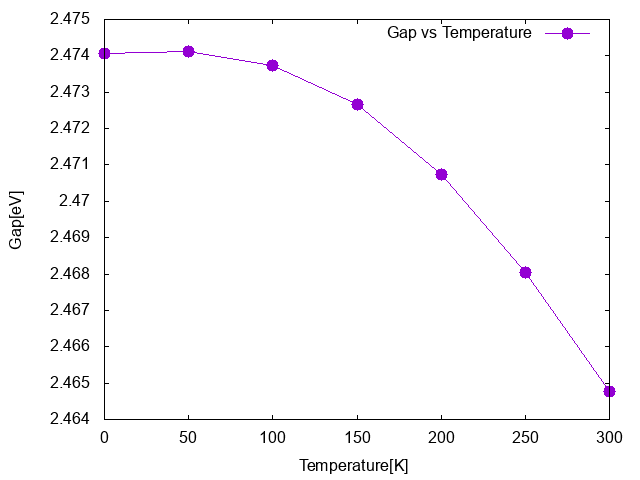
run again yambo_ph -J T300 and compare the two output file o-T0.qp and o-T300.qp, to find how much the gap change with the temperature. If you repeat the calculation for different temperature you can obtain the trend of the gap vs temperature. The figure below report the Silicon gap at Gamma Point at different temperature obtained in this tutorial:
If you uncomment the flag WRgFsq the code saves information about the Eliashberg functions that can be plotted using the ypp_ph, see below.
Finally if you add -V qp in the input generation a new flag appears OnMassShell, if you un-comment this flag calculation will be performed in the "on mass shell" approximation, namely the static limit the Quasi-Particle approximation, for a discussion see reference [2]
Notice that the last column in the quasi-particle file "o.QP" contains the quasi-particle width, that is related to their life-time. You can plot the band structure including this width to get quasi-particle spectra
similar to the one measured in ARPES experiments, see Fig. 2 in ref. [3].
This parameter will be used in the next tutorial on optical properties at finite temperature.
WARNING: Yambo average the electron-phonon correction on the degenerate states, please include all degenerate states in your calculations. For example in the silicon case you need correction from the 2nd band to the 8th band.
Convergence
The results of this tutorial are not converged. This is due to the poor parameters used in this tutorial to make the calculations fast. In order to have converged results, first of all you have to be sure to have converged phonons, in order to do that increase plane-wave cutoff, number of k-points and if necessary reduce tr2_ph.
Then change the parameters for the Yambo calculations, increasing the number of k and q points and the number of bands. If you want to increase only the number of bands, just repeat the nscf and dvscf calculations without recalculate phonons. In the following section we will describe a smart way to accelerate convergence.
Nota bene: At present Yambo neither implements the Fröhlich term at q=0[4] nor the quadrupolar correction,[5] therefore convergence in polar material can be very slow with the number of q-points.
Double-grid method for the electron-phonon coupling (only in Yambo 5.x)
Simplifying at most the matrix elements of the electron-phonon self-energy have the structure:
where we omitted the electronic band and the phonon branches indexes. In order to speed up calculation one can average the denominators on an additional fine grid around each q points as:
In order to exploit the double-grid tool we need the phonon energies calculated on a fine grid. If you just want to test the functionality of Yambo you can download here some files with the phononic frequencies already calculated on different silicon grids: si_freqs_files.tgz
Otherwise you generate them by following the instructions below.
For a general tutorial on phonon calculation with Quantum Espresso you can have a look at Hands on phonons.
Starting from a well converged phonon calculation matdyn.x can interpolate phonon dispersion on a given q-sampling (for example a regular 14x14x14 grid, as shown in the input file below) and give the desired phonon energies.
&input
    asr='simple',
    flfrc='si.fc',
    flfrq='si.freq',
    dos=.true.,
    fldos='si.dos',
    deltaE=1.d0,
    nk1=14, nk2=14, nk3=14
/
Alternatively you can generate a random q-sampling using Yambo (ypp -k r) and insert the corresponding q points list into a matdyn file.
Once you generated the phonon energies you can read them with the command ypp_ph -g d:
gkkp                             # [R] gkkp databases
gkkp_dg                          # [R] GKKP double grid
PHfreqF= "si.freq"            # PWscf format file containing the phonon frequencies
PHmodeF= "none"                  # PWscf format file containing the phonon modes
FineGd_mode= "mixed"             # Fine Grid mode. Symmetry expanded, unexpanded or mixed.
#SkipBorderPts                 # Skip points in the Fine Grid that are on the surface of coarse gride smal BZ`s
EkplusQmode= "interp"            # E(k+q) energies calculation mode (interp | dftp )
#TestPHDGrid                   # Test double-grid: set all values of the fine grid equal to the couse ones
then run ypp_ph an it will generate a new file SAVE/ndb.PH_Double_Grid.
In the calculation the new phonon energies will be expanded
using the symmetries of the systems, while the electronic energies at k+q will be interpolated using a smooth Fourier interpolation[6].
In order to perform calculation with the double grid remove the SAVE/ndb.QP file and repeat the calculation.
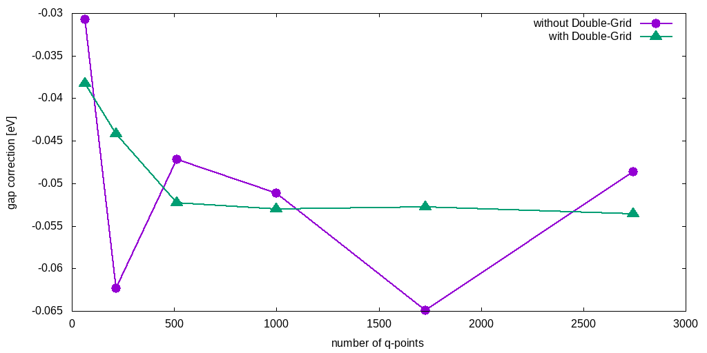
The best strategy to converge electron-phonon coupling calculations is to converge the double-grid for a fixed course grid and the increase the second one. Hereafter an example of Silicon band gap correction convergence versus the number of q-points in the course grid, using a double-grid with 4096 random q-points.
The double-grid implementation is described in this paper[7].
Miscellaneous and post-processing
Automatic generation of electron-phonon matrix elements
Getting electron-phonon matrix elements from QuantumEspresso to Yambo is a complicated process,
we advice you to create a script to automatize the procedure, here an example of a bash script for the silicon case: SILICON-SCRIPT.
There are a list of utilities to analyze electron-phonon coupling results:
Phonon density of states
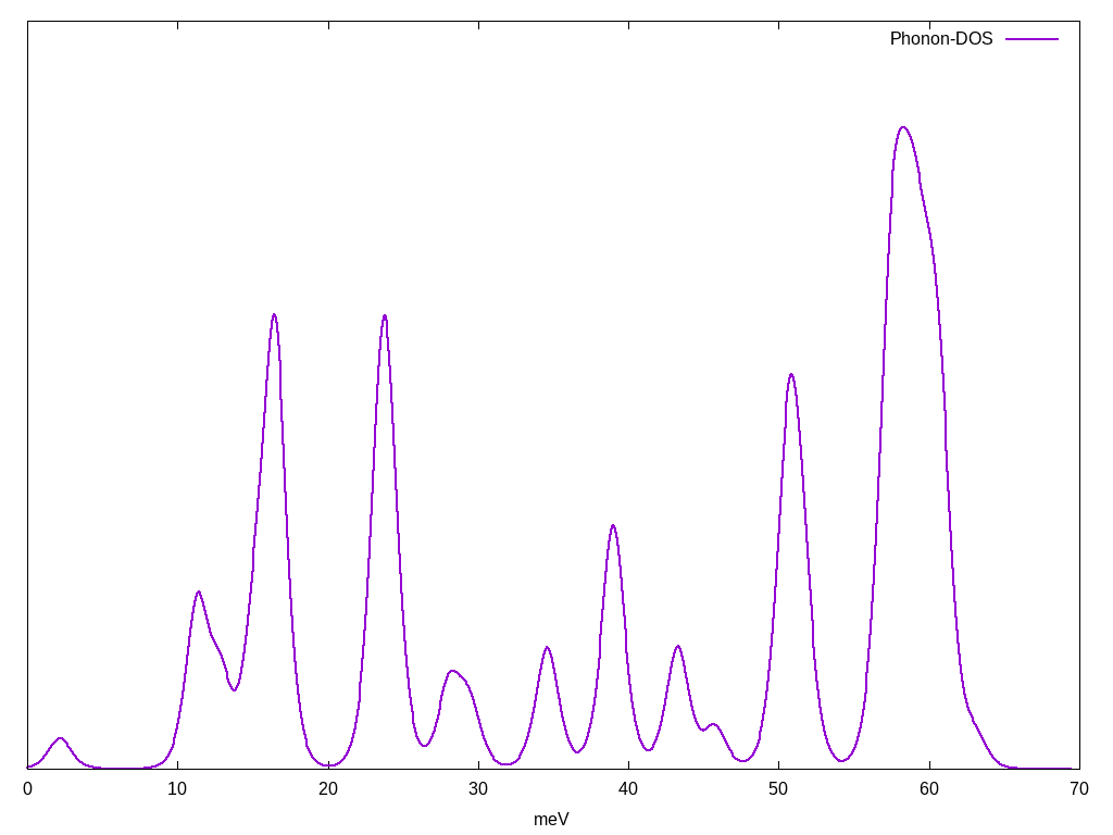
You can plot phonon density of states with the command: ypp_ph -p d. In order to get a nice plot set in the input
phonons                          # [R] Phononic properties
dos                              # [R] DOS
PhBroad= 0.0005000          eV    # Phonon broadening (Eliashberg & DOS)
PhStps=1000                      # Energy steps
notice that this is an easy quantity to check for the convergence in q-points.
Eliashberg Functions
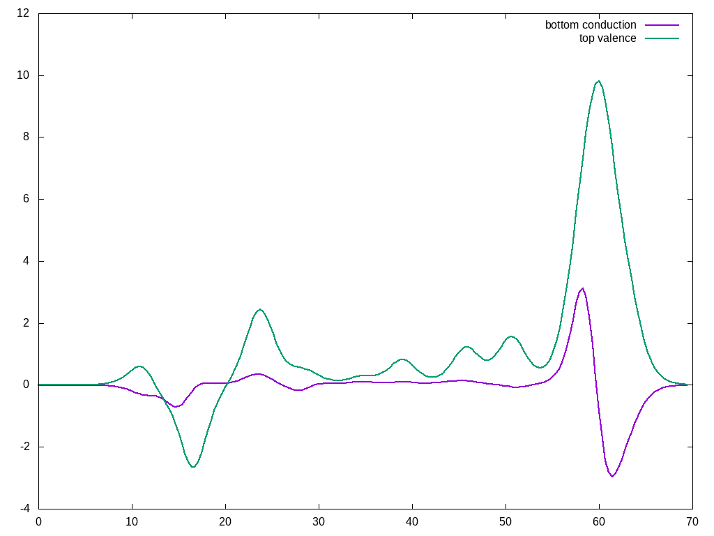
You can plot Eliashberg functions[8] for both electrons and excitons. In order to plot Eliashberg functions you must have calculated Quasi-Particle correction with the flag WRgFsq, see above.
The command ypp_ph -s e generate the input for the electronic Eliashberg functions:
electrons                        # [R] Electronic properties
eliashberg                       # [R] Eliashberg
PhBroad= 0.0010000          eV    # Phonon broadening (Eliashberg & DOS)
PhStps= 200                      # Energy steps
%QPkrange                        #  generalized Kpoint/Band indices
 1|1|4|5|
%
in this example we plot Eliashberg functions for the top valence and bottom conduction band at Gamma point:
For a discussion on how to interprete Eliashberg functions and use them to understand the different phonon contribution you can have a look to ref.[9]
Atomic displacement amplitudes
Running ypp_ph -p a will plot the atomic displacement for each atom in the cell each direction.
Other variables in the input files
In the input files of the present tutorial there are other variable not used in this tutorial.
In particular GkkpExpand is used for other calculations not present in the GPL, while GkkpConvert is used to checking purpose the IO for different versions
of the databases.
Links
- Back to ICTP 2022#Tutorials
References
- ↑ This tutorial is based on Elena Cannuccia blog
- ↑ H. Kawai et al. Phys. Rev. B 89, 085202 (2014)
- ↑ G. Antonius, S. Poncé, E. Lantagne-Hurtubise, G. Auclair, X. Gonze, and M. Côté Phys. Rev. B 92, 085137 (2015)
- ↑ Carla Verdi and Feliciano Giustino Phys. Rev. Lett. 115, 176401 (2015)
- ↑ G. Brunin et al. Phys. Rev. Lett. 125, 136601 (2020)
- ↑ Warren E. Pickett, Henry Krakauer, and Philip B. Allen, Phys. Rev. B 38, 2721(1988)
- ↑ Double-grid for the electron-phonon problem, (to be published) E. Cannuccia, C. Attaccalite and V. Olevano (2022)
- ↑ F. Marsiglio, J.P. Carbotte Electron - Phonon Superconductivity
- ↑ E. Cannuccia and A. Gali Phys. Rev. Materials 4, 014601 (2020)
