Real time approach to linear response

In this example, we will consider a single layer of hexagonal boron nitride (hBN). If you didn't before you can download input files and Yambo databases for this tutorial here: hBN-2D-RT.tar.gz. and/or follow the instructions to generate the databases here: Prerequisites for Real Time propagation with Yambo

Real-time dynamics at the independent particles level

Since we work with the two independent approaches coded in yambo it will be useful to create two different folders for the input files.

mkdir Inputs_rt
mkdir Inputs_nl

In order to calculate linear-response in real-time, we will perturb the system with a delta function in time external field.

Approach based on the density matrix

Use the command yambo_rt -p p -F 01_td_ip.in to generate the input:

 negf                           # [R] Real-Time dynamics
 RT_Threads=0                   # [OPENMP/RT] Number of threads for real-time
 HXC_Potential= "IP"           # [SC] SC HXC Potential
 % RTBands
   3 |  6 |                     # [RT] Bands
 %
 Integrator= "EULER RK2"              # [RT] Integrator. Use keywords space separated  ( "EULER/EXPn/INV" "SIMPLE/RK2/RK4/HEUN" "RWA")
 PhLifeTime= 0.000000   fs      # [RT] Dephasing Time
 RTstep=10.000000       as      # [RT] Real Time step length
 NETime= 55.00000       fs      # [RT] Simulation Time
 % IOtime
  0.05     | 5.00     | 0.10     |  fs    # [RT] Time between to consecutive I/O (OBSERVABLEs,CARRIERs - GF - OUTPUT)
 %
 % Field1_Freq
  0.00     | 0.00     | eV      # [RT Field1] Frequency
 %
 Field1_Int=1.E4   kWLm2   # [RT Field1] Intensity
 Field1_Width= 0.000000 fs      # [RT Field1] Width
 Field1_kind= "DELTA"           # [RT Field1] Kind(SIN|RES|ANTIRES|GAUSS|DELTA|QSSIN)
 Field1_pol= "linear"           # [RT Field1] Pol(linear|circular)
 % Field1_Dir
  0.000000 | 1.000000 | 0.000000 |        # [RT Field1] Versor
 %
 % Field1_Dir_circ
  0.000000 | 1.000000 | 0.000000 |        # [RT Field1] Versor_circ
 %
 Field1_Tstart= 0.000000fs      # [RT Field1] Initial Time

Set the field direction along y, the field type to DELTA, the length of the simulation to 55 fs, number of bands from 3 to 6, dephasing to zero and the field intensity to 1.E4. The yambo_rt is optimized for TD-SEX (or even more sophisticated calculations). The I/O time, which is negligible in such calculations, is less optimized and becomes the most time demanding step here. We can overcome this setting the IOtime for the polarization to 50 as (i.e. each 5 time steps).

Approach based on the Berry Phase

Use the command yambo_nl -u -F input_lr.in to generate the input:

nlinear                      # [R NL] Non-linear optics
NL_Threads= 1                # [OPENMP/NL] Number of threads for nl-optics
% NLBands
  3 |  6 |                   # [NL] Bands
%
NLstep=   0.0100       fs    # [NL] Real Time step length
NLtime=55.000000      fs    # [NL] Simulation Time
NLverbosity= "high"           # [NL] Verbosity level (low | high)
NLintegrator= "INVINT"       # [NL] Integrator ("EULEREXP/RK4/RK2EXP/HEUN/INVINT/CRANKNIC")
NLCorrelation= "IPA"         # [NL] Correlation ("IPA/HARTREE/TDDFT/LRC/JGM/SEX/HF")
NLLrcAlpha= 0.000000         # [NL] Long Range Correction
% NLEnRange
 0.200000 | 8.000000 | eV    # [NL] Energy range 
%
NLEnSteps= 1                 # [NL] Energy steps
NLDamping= 0.000000    eV    # [NL] Damping
% ExtF_Dir
 0.000000 | 1.000000  | 0.000000 |        # [NL ExtF] Versor
%
ExtF_kind=  "DELTA"          # [NL ExtF] Kind(SIN|SOFTSIN|RES|ANTIRES|GAUSS|DELTA|QSSIN)

The standard input of yambo_nl is thought for the non-linear response so we have to change some parameters in order to calculate the linear response. Set the field direction along y, the field type to DELTA, the length of the simulation to 55 fs, number of bands from 3 to 6 dephasing to zero and the number of energy steps to one, as shown above in red. We set the verbosity to "high" in such a way to print real-time output files. We set the differential equation integrator to INVINT that is faster but less accurate than the default (see Ref. ) . This integrator is ok in case of independent particles but I advise you to use CRANKNIC integrator when correlation effects are present. 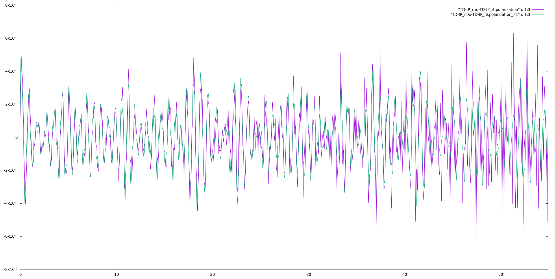Now run yambo_nl -F input_lr.in The code will produce different files: o.polarization_F1 that contains the polarization, o.external_potential_F1 the external field we used, and finally r_optics_nloptics a report with all information about the simulation. If you plot the third column of o.polarization_F1 versus the first one (time-variable) you will get the time-dependent polarization along the y-direction:

Results Analysis

Now we can use ypp_nl -u to analyze the results:

nonlinear                    # [R] NonLinear Optics Post-Processing
Xorder= 1                    # Max order of the response functions
% TimeRange
-1.000000 |-1.000000 | fs    # Time-window where processing is done
%
ETStpsRt= 1001                # Total Energy steps
% EnRngeRt
  0.00000 | 10.00000 | eV    # Energy range
%
DampMode= "LORENTZIAN"             # Damping type ( NONE | LORENTZIAN | GAUSSIAN )
DampFactor=  0.10000   eV    # Damping parameter

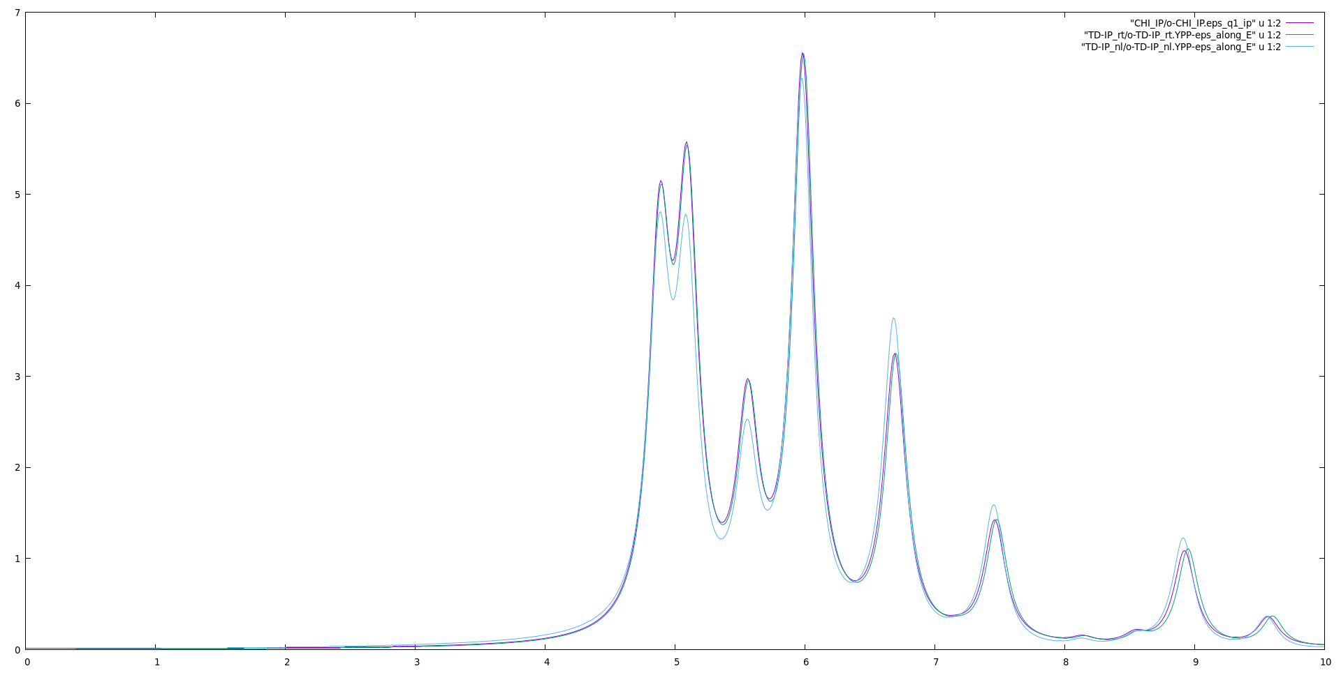
where we set a Lorentzian smearing corresponding to 0.1 eV. Notice that due to the finite time of our simulation smearing is always necessary to Fourier transform the result. Then we run ypp_nl and obtain the following files: the dielectric constant along with the field direction o.YPP-eps_along_E, the EELS along with the same direction o.YPP-eels_along_E, and the damped polarization o.YPP-damped_polarization. Now we can plot the dielectric constant and compare it with the linear response:

The input for the linear response can be downloaded here.