Pump and Probe: Difference between revisions
| Line 210: | Line 210: | ||
PumpPATH= "<span style="color:red">./PUMP/</span>" # Path of the simulation with the Pump only | PumpPATH= "<span style="color:red">./PUMP/</span>" # Path of the simulation with the Pump only | ||
Notice that in this case we are interested in the spectra below the 4 eV, that is was zero without the presence of the pump. We put in the input the pump path in such way to calculate the | Notice that in this case we are interested in the spectra below the 4 eV, that is was zero without the presence of the pump. We put in the input the pump path in such way to calculate the | ||
<math>\Delta P(t) = P_{PnP}(t) - P_{pump}(t) | |||
</math>. | |||
== References == | == References == | ||
Revision as of 16:15, 8 November 2022
This tutorial works only with Yambo version > 5.1, that will be released soon.
In this tutorial we will show you how to setup two external fields in yambo_nl, to perform pump and probe simulation. [1]
This tutorial is at independent particle level, but the same kind of simulation can be repeated including local field effects,
quasi-particle correction or electron-hole interaction, see for example the tutorials:
Correlation effects in the non-linear response
Real time Bethe-Salpeter Equation (TDSE)
This tutorial supposes that you are already familiar with real-time simulation with Yambo[2]
if it is not the case please check these tutorials: Tutorials#Non_linear_response
We start from the h-BN monolayer with an in place lattice constant a=2.5 Å and a box large 30 a.u. in the z-direction.
Standard DFT input for hBN monolayer for ABINIT or QuantumEspresso can be found here Tutorials.
We used a 9x9x1 k-points grid and 8 bands in the non-self consistent calculation.
In our example we choose direction [0,1,0] for the pump and [1,0,0] for the probe. We generate the ypp.in to remove symmetries with the command ypp -y and we modify it as:
fixsyms                          # [R] Remove symmetries not consistent with an external perturbation
% Efield1
 0.000000 | 1.000000 | 0.000000 |        # First external Electric Field
%
% Efield2
 1.000000 | 0.000000 | 0.000000 |        # Additional external Electric Field
%
BField= 0.000000           T     # [MAG] Magnetic field modulus
Bpsi= 0.000000             deg   # [MAG] Magnetic field psi angle [degree]
Btheta= 0.000000           deg   # [MAG] Magnetic field theta angle [degree]
#RmAllSymm                     # Remove all symmetries
RmTimeRev                     # Remove Time Reversal
#RmSpaceInv                    # Remove Spatial Inversion
then we go in the FixSymm directory and run again the setup.
We will perform three different real-time calculations:
- the probe field alone;
- the pump field alone;
- the pump and probe configuration.
Probe only
We can generate the input file for a generic Pump and Probe calculations with the command: yambo_nl -u p -F yambo.in_probe:
nloptics                         # [R] Non-linear spectroscopy
DIP_Threads=0                    # [OPENMP/X] Number of threads for dipoles
NL_Threads=0                     # [OPENMP/NL] Number of threads for nl-optics
% NLBands
    3 |  6 |                           # [NL] Bands range
%
NLverbosity= "high"              # [NL] Verbosity level (low | high)
NLtime=  80.000000           fs    # [NL] Simulation Time
NLintegrator= "  CRANKNIC"           # [NL] Integrator ("EULEREXP/RK2/RK4/RK2EXP/HEUN/INVINT/CRANKNIC")
NLCorrelation= "IPA"             # [NL] Correlation ("IPA/HARTREE/TDDFT/LRC/LRW/JGM/SEX")
NLLrcAlpha= 0.000000             # [NL] Long Range Correction
NLDamping= 0.000000        eV    # [NL] Damping (or dephasing)
RADLifeTime=-1.000000      fs    # [RT] Radiative life-time (if negative Yambo sets it equal to Phase_LifeTime in NL)
#EvalCurrent                   # [NL] Evaluate the current
#FrPolPerdic                   # [DIP] Force periodicity of polarization respect to the external field
HARRLvcs= 21817            RL    # [HA] Hartree     RL components
EXXRLvcs= 21817            RL    # [XX] Exchange    RL components
% Field1_Freq
 0.100000 | 0.100000 |         eV    # [RT Field1] Frequency
%
Field1_NFreqs= 1                 # [RT Field1] Frequency
Field1_Int=  1000.00       kWLm2 # [RT Field1] Intensity
Field1_Width= 0.000000     fs    # [RT Field1] Width
Field1_kind= "  DELTA"           # [RT Field1] Kind(SIN|COS|RES|ANTIRES|GAUSS|DELTA|QSSIN)
Field1_pol= "linear"             # [RT Field1] Pol(linear|circular)
% Field1_Dir
   0.000000 | 1.000000 | 0.000000 |        # [RT Field1] Versor
%
Field1_Tstart=   5.00000    fs    # [RT Field1] Initial Time
[......]
In this input we set only the first field that is the probe, we use a DELTA function as field in such a way to probe all the frequencies, and set the starting point of the delta at t=5 fs.
Run this job in a separate folder with the command yambo_nl -F yambo.in_probe -J PROBE. Then we can analyze the spectra with ypp -u -J PROBE :
nonlinear                        # [R] Non-linear response analysis
Xorder= 1                        # Max order of the response/exc functions
% TimeRange
-1.000000 |-1.000000 |         fs    # Time-window where processing is done
%
ETStpsRt= 200                    # Total Energy steps
% EnRngeRt
  0.00000 | 20.00000 |         eV    # Energy range
%
DampMode= "LORENTZIAN"           # Damping type ( NONE | LORENTZIAN | GAUSSIAN )
DampFactor= 0.100000       eV    # Damping parameter
PumpPATH= "none"           # Path of the simulation with the Pump only
and get the dielectric response. Notice that we introduce a Lorentzian broadening the post-processing.
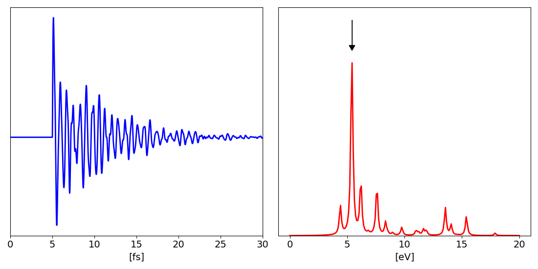
Hereafter we plot the damped polarization along the y-direction and the corresponding dielectric constant:
the arrow indicates the position where we will put the Pump in the next simulation.
Pump only
Now we run a simulation with the pump field only. We generate the input in the same way yambo_nl -u p -F yambo.in_pump.
These result will be our reference field in the final analysis. Here the input file for the pump:
nloptics                         # [R] Non-linear spectroscopy
DIP_Threads=0                    # [OPENMP/X] Number of threads for dipoles
NL_Threads=0                     # [OPENMP/NL] Number of threads for nl-optics
% NLBands
   3 |  6 |                           # [NL] Bands range
%
NLverbosity= "high"              # [NL] Verbosity level (low | high)
NLtime=  150.0000           fs    # [NL] Simulation Time
NLintegrator= "CRANKNIC"         # [NL] Integrator ("EULEREXP/RK2/RK4/RK2EXP/HEUN/INVINT/CRANKNIC")
NLCorrelation= "IPA"             # [NL] Correlation ("IPA/HARTREE/TDDFT/LRC/LRW/JGM/SEX")
NLLrcAlpha= 0.000000             # [NL] Long Range Correction
NLDamping= 0.000000        eV    # [NL] Damping (or dephasing)
RADLifeTime=-1.000000      fs    # [RT] Radiative life-time (if negative Yambo sets it equal to Phase_LifeTime in NL)
#EvalCurrent                   # [NL] Evaluate the current
#FrPolPerdic                   # [DIP] Force periodicity of polarization respect to the external field
HARRLvcs= 21817            RL    # [HA] Hartree     RL components
EXXRLvcs= 21817            RL    # [XX] Exchange    RL components
% Field1_Freq
 0.100000 | 0.100000 |         eV    # [RT Field1] Frequency
%
Field1_NFreqs= 1                 # [RT Field1] Frequency
Field1_Int=  10000.00       kWLm2 # [RT Field1] Intensity
Field1_Width= 0.000000     fs    # [RT Field1] Width
Field1_kind= "SOFTSIN"           # [RT Field1] Kind(SIN|COS|RES|ANTIRES|GAUSS|DELTA|QSSIN)
Field1_pol= "linear"             # [RT Field1] Pol(linear|circular)
% Field1_Dir
 0.000000 | 0.000000 | 0.000000 |        # [RT Field1] Versor
%
Field1_Tstart= 0.010000    fs    # [RT Field1] Initial Time
% Field2_Freq
  5.42 | 5.42 |         eV    # [RT Field2] Frequency
%
Field2_NFreqs= 1                 # [RT Field2] Frequency
Field2_Int=  1000.00       kWLm2 # [RT Field2] Intensity
Field2_Width= 10.00000     fs    # [RT Field2] Width
Field2_kind= "QSSIN"             # [RT Field2] Kind(SIN|COS|RES|ANTIRES|GAUSS|DELTA|QSSIN)
Field2_pol= "linear"             # [RT Field2] Pol(linear|circular)
% Field2_Dir
 0.000000 | 1.000000 | 0.000000 |        # [RT Field2] Versor
%
Field2_Tstart= 0.010000    fs    # [RT Field2] Initial Time
[...]
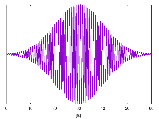
In this simulation we used as Pump field QSSIN that is sinus with a Guassian envelopesine-Gaussian wave. For a list of all possible field in Yambo see the file src/modules/mod_fields.F. We centred the field frequency at 5.22 eV that is the energy of the highest peak in the previous figure, see arrow there. Run the simulation with the command yambo_nl -F yambo.in_pump -J PUMP . The pump field (column 6th of the file o-PUMP.external_potential_F1) is shown in the figure below:
Pump and probe
Now we copy the pump in file in a new file cp yambo.in_pump yambo.in_pump_and_probe and turn on the probe field:
nloptics                         # [R] Non-linear spectroscopy
DIP_Threads=0                    # [OPENMP/X] Number of threads for dipoles
NL_Threads=0                     # [OPENMP/NL] Number of threads for nl-optics
% NLBands
  3 |  6 |                           # [NL] Bands range
%
NLverbosity= "high"              # [NL] Verbosity level (low | high)
NLtime=  150.0000           fs    # [NL] Simulation Time
NLintegrator= "CRANKNIC"         # [NL] Integrator ("EULEREXP/RK2/RK4/RK2EXP/HEUN/INVINT/CRANKNIC")
NLCorrelation= "IPA"             # [NL] Correlation ("IPA/HARTREE/TDDFT/LRC/LRW/JGM/SEX")
NLLrcAlpha= 0.000000             # [NL] Long Range Correction
NLDamping= 0.000000        eV    # [NL] Damping (or dephasing)
RADLifeTime=-1.000000      fs    # [RT] Radiative life-time (if negative Yambo sets it equal to Phase_LifeTime in NL)
#EvalCurrent                   # [NL] Evaluate the current
#FrPolPerdic                   # [DIP] Force periodicity of polarization respect to the external field
HARRLvcs= 21817            RL    # [HA] Hartree     RL components
EXXRLvcs= 21817            RL    # [XX] Exchange    RL components
% Field1_Freq
 0.100000 | 0.100000 |         eV    # [RT Field1] Frequency
%
Field1_NFreqs= 1                 # [RT Field1] Frequency
Field1_Int=  1.00       kWLm2 # [RT Field1] Intensity
Field1_Width= 0.000000     fs    # [RT Field1] Width
Field1_kind= "DELTA"           # [RT Field1] Kind(SIN|COS|RES|ANTIRES|GAUSS|DELTA|QSSIN)
Field1_pol= "linear"             # [RT Field1] Pol(linear|circular)
% Field1_Dir
 1.000000 | 0.000000 | 0.000000 |        # [RT Field1] Versor
%
Field1_Tstart= 90.0000    fs    # [RT Field1] Initial Time
% Field2_Freq
  5.42 | 5.42 |         eV    # [RT Field2] Frequency
%
Field2_NFreqs= 1                 # [RT Field2] Frequency
Field2_Int=  1000.00       kWLm2 # [RT Field2] Intensity
Field2_Width= 10.00000     fs    # [RT Field2] Width
Field2_kind= "QSSIN"             # [RT Field2] Kind(SIN|COS|RES|ANTIRES|GAUSS|DELTA|QSSIN)
Field2_pol= "linear"             # [RT Field2] Pol(linear|circular)
% Field2_Dir
 0.000000 | 1.000000 | 0.000000 |        # [RT Field2] Versor
%
Field2_Tstart= 0.010000    fs    # [RT Field2] Initial Time
you run the simulation with the command yambo_nl -F yambo.in_pump_and_probe -J PUMP_AND_PROBE and then we analyze the result using ypp with the command: ypp_nl -u -J PUMP_AND_PROBE :
nonlinear                        # [R] Non-linear response analysis
Xorder= 1                        # Max order of the response/exc functions
% TimeRange
-1.000000 |-1.000000 |         fs    # Time-window where processing is done
%
ETStpsRt= 500                    # Total Energy steps
% EnRngeRt
  0.00000 | 3.9000 |         eV    # Energy range
%
DampMode= "GAUSSIAN"                 # Damping type ( NONE | LORENTZIAN | GAUSSIAN )
DampFactor= 0.085000       eV    # Damping parameter
PumpPATH= "./PUMP/"                 # Path of the simulation with the Pump only
Notice that in this case we are interested in the spectra below the 4 eV, that is was zero without the presence of the pump. We put in the input the pump path in such way to calculate the [math]\displaystyle{ \Delta P(t) = P_{PnP}(t) - P_{pump}(t) }[/math].
References
- ↑ Exciton - Exciton transitions involving strongly bound Frenkel excitons: an ab initio approach, D. Sangalli, M. D'Alessandro and C. Attaccalite, in preparation
- ↑ Non-linear response in extended systems: a real-time approach, C. Attaccalite

