Optics at the independent particle level

In this tutorial you will learn how to calculate optical spectra at the RPA or independent particle level for bulk hBN.

Prerequisites

• You must first complete the "How to use Yambo" tutorial

You will need:

• The SAVE databases for bulk hBN
• The yambo executable
• gnuplot, for plotting spectra

Choosing input parameters

Enter the folder for bulk hBN that contains the SAVE directory, and generate the input file. From yambo -H you should understand that the correct option is yambo -o c. Let's add some command line options:

$ cd YAMBO_TUTORIALS/hBN/YAMBO
$ yambo -o c -F yambo.in_IP -J Full

This corresponds to optical properties in G-space at the independent particle level (Chimod= "IP"). Let's calculate just for the long-wavelength limit q = 0. This always corresponds to the first q-point. Change the following variables in the input file to:

% QpntsRXd
 1 |  1 |                   # [Xd] Transferred momenta
%
ETStpsXd= 1001               # [Xd] Total Energy steps

in order to select just the first q. The last variable ensures we generate a smooth spectrum. Save the input file and launch the code, keeping the command line options as before (i.e., just remove the lower case options):

$ yambo -F yambo.in_IP -J Full
...
 <---> [05] Optics
<---> [LA] SERIAL linear algebra
<---> [DIP] Checking dipoles header
<---> [x,Vnl] computed using 4 projectors
<---> [M  0.017 Gb] Alloc WF ( 0.016)
<---> [WF] Performing Wave-Functions I/O from ./SAVE
<01s> Dipoles: P and iR (T): |########################################| [100%] 01s(E) 01s(X)
<01s> [M  0.001 Gb] Free WF ( 0.016)
<01s> [DIP] Writing dipoles header
<01s> [X-CG] R(p) Tot o/o(of R)  :   5501   52992     100
<01s> Xo@q[1] |########################################| [100%] --(E) --(X)
<01s> [06] Game Over & Game summary
$ ls
Full   SAVE  yambo.in_IP   r_setup
o-Full.eel_q1_ip  o-Full.eps_q1_ip  r-Full_optics_chi

Let's take a moment to understand what Yambo has done in side the Optics runlevel:

1. Compute the [x,Vnl] term
2. Read the wavefunctions from disc [WF]
3. Compute the dipoles, i.e. matrix elements of p
4. Write the dipoles to disk as SAVE/ndb.dip* databases. This you can see in the report file:

$ grep -A20 "WR" r-Full_optics_chi 
[WR./Full//ndb.dip_iR_and_P]
Brillouin Zone Q/K grids (IBZ/BZ):  14   72   14   72
RL vectors                   (WF): 1491
Electronic Temperature        [K]: 0.0000000
Bosonic    Temperature        [K]: 0.0000000
X band range           :   1  100
RL vectors in the sum  : 1491
[r,Vnl] included       :yes
...

4. Finally, Yambo computes X₀ for this q, and writes the dielectric function inside the o-Full.eps_q1_ip file for plotting

Before plotting the output, let's change a few more variables. The previous calculation used all the G-vectors in expanding the wavefunctions, 1491. This corresponds roughly to the cut off energy of 40Ry we used in the DFT calculation. Generally, however, we can use a smaller value. We use the verbosity to switch on this variable, and a new -J flag to avoid reading the previous database:

$ yambo -o c -F yambo.in_IP -J 6Ry -V RL

Change the value of FFTGvecs and its unit:

FFTGvecs= 6           Ry    # [FFT] Plane-waves

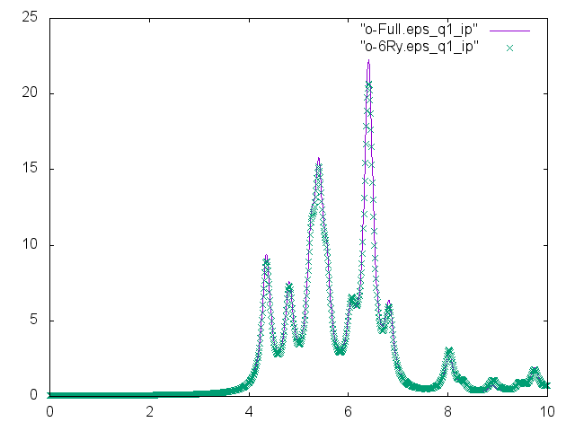
Save the input file and launch the code again, and then plot the o-Full.eps_q1_ip and o-6Ry.eps_q1_ip files:

$ gnuplot
gnuplot> plot "o-Full.eps_q1_ip" w l,"o-6Ry.eps_q1_ip" w p

Clearly there is very little difference between the two spectra. Last, let's select a different component of the dielectric tensor:

$ yambo -o c -F yambo.in_IP -J 6Ry -V RL
...
% LongDrXd
0.000000 | 0.000000 | 1.000000 |        # [Xd] [cc] Electric Field
%
...
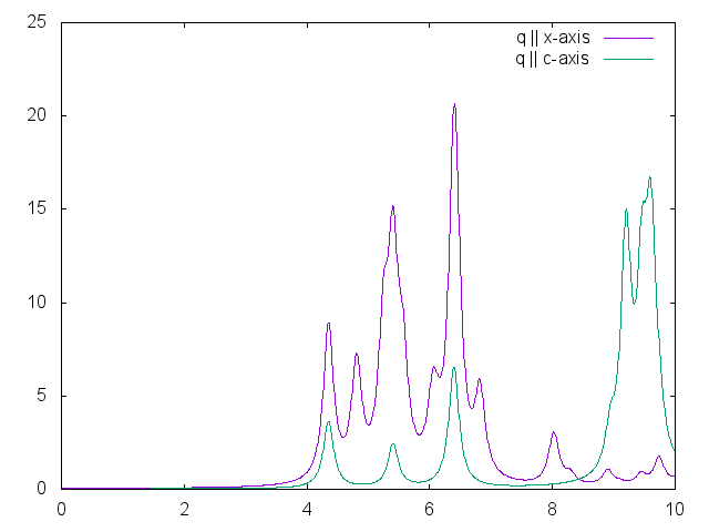
$ yambo -F yambo.in_IP -J 6Ry -V RL

This time yambo reads from the 6Ry folder, so it does not need to compute the dipoles again. Plotting gives:

$ gnuplot
gnuplot> plot "o-6Ry.eps_q1_ip" t "q || x-axis" w l,"o-6Ry.eps_q1_ip_01" t "q || c-axis" w l