Hartree Fock

Prerequisites

Cheatsheet on HF

• You must first complete the "How to use Yambo" modules (input file generation and command_line_options, Initialization)

You will need:

• The SAVE databases for bulk hBN
• The yambo executable
• gnuplot for plotting spectra

Background

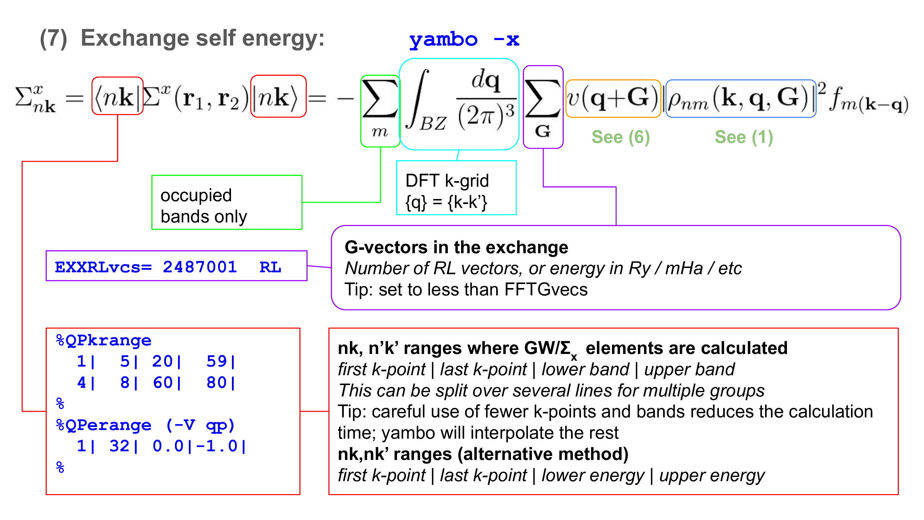
The exchange part contribution of the self-energy for a generic state (nk) in reciprocal space reads:

It is important to note that in this way we are adding the HF contribution in a perturbative way to previously calculated DFT energies:

and hence they will differ from a standard self-consistent HF calculation.

Input file generation

Let's start by building up an input file for a HF calculation. From yambo -h you should understand that the correct option is yambo -x:

$ cd YAMBO_TUTORIALS/hBN/YAMBO
$ yambo        (Initialization)
$ yambo -x -F hf.in

Looking inside the input file you will find:

EXXRLvcs = 3187        RL    # [XX] Exchange RL components
VXCRLvcs = 3187        RL    # [XC] XCpotential RL components
%QPkrange                    # [GW] QP generalized Kpoint/Band indices
  1| 14|  1|100|
%

The variable EXXRLvcs governs the number of G vectors to be summed in the expression of the exchange self-energy reported above. The variable VXCRLvcs set the number of G vectors used in the evaluation of the density for the <Vxc> matrix element. A large number is needed in order to have a precise cancellation with the ground state calculation, in particular when GGA potentials are used. A good practice is to leave it at the maximum number (default). In case it would be needed to reduce (e.g. for memory reason), the accuracy can be checked by comparing the E_xc value printed in Yambo report and QE output file. The QPkrange name list it is a generalized index needed to select the first and last kpoints and bands we want to calculate the QP correction. In general, we are interested in the gap of the system or in the band structure across the Fermi Energy. Let's start by editing the hf.in file by selecting the last occupied and first unoccupied bands These are the bands 8 and 9 as reported in the r_setup file. So we change the QPkrange variable in:

%QPkrange                    # [GW] QP generalized Kpoint/Band indices
   1| 14|  8| 9|
%

and run calculations to converge the expression above. In the expression of the Exchange Self Energy, we have a summation over bands, an integral over the Brillouin Zone and a Sum over the G vectors. Looking at the occupation factor we realize that occupied states only enters in the expression, so we do not need to worry about the bands as Yambo will include all the occupied bands by default. In order to check convergence of the G vectors in the summation in the Σx expression, we will perform different calculation varying the kinetic energy cutoff governing the number of G vectors entering in the sum. Let's start by setting in hf.in:

EXXRLvcs= 10 Ry

Calculation and analysis of output

Let's now run yambo:

$ yambo -F hf.in -J 3D

The result can be found int the output o-3D.hf file and in the r-3D_HF_and_locXC file. Looking inside the output file we have:

#  K-point          Band       Eo           Ehf          DFT        HF
#
    1.00000      8.00000     -1.29642     -4.79324    -18.03344    -21.53026
    1.00000      9.00000      4.83239     9.755507    -9.592554    -4.669446
    2.00000      8.00000     -1.33551     -4.80994    -18.07476    -21.54919
    2.00000      9.00000      7.56742     13.43122    -11.55012    -5.68633
........

Looking at the definition of the HF energy, the third column is the DFT energy (KS eigenvalue), Ehf is the HF energy, and column 4 and 5 report the different contribution to be subtracted Vx (DFT) and added Σx (HF) to the unperturbed DFT eigenvalue. From these data we can calculate the HF gap: you can recognize that the direct gap is found at k-point number 7, being 4.29 eV at DFT level and 11.95 eV in HF approximation. This information can be also easily found in the report file r-3D_HF_and_locXC searching for Direct Gaps:

Before the HF computation:

 [X] Direct Gap                                    :  4.289853 [eV]
 [X] Direct Gap localized at k-point               :   7
 [X] Indirect Gap                                  :  3.877976 [eV]
 [X] Indirect Gap between k-points                 :  14   7

... after the HF computation:

[05.01] HF occupations report
 =============================

 [Hartree-Fock] Direct Gap                         :  11.94549 [eV]
 [Hartree-Fock] Direct Gap localized at k-point    :   7
 [Hartree-Fock] Indirect Gap                       :  11.28767 [eV]
 [Hartree-Fock] Indirect Gap between k-points      :  14   7

or simply by typing:

$ grep "Direct Gap" r-3D_HF_and_locXC

and the gap value before and after the HF correction is shown:

 [X] Direct Gap                                    :  4.289853 [eV]
 [X] Direct Gap localized at k-point               :   7
 [Hartree-Fock] Direct Gap                         :  11.94549 [eV]
 [Hartree-Fock] Direct Gap localized at k-point    :   7

In the report file, the first value indicates the minimum gap while the second one is the maximum energy gap between the same bands.

In the following, in order to converge the direct gap, we will focus the K point where the direct band is found. Inspecting the r_setup file, or any other report file it can be recognized that the direct minimum gap is found at the K-point number 7 (M point): this can be seen by searching the DFT "Direct Gap" and looking at the eigenvalues reported for each k point. Note that the zero energy is fixed at the top of the valence band, K point number 14 (H point). So we can restrict the convergence calculations to the occupied and empty bands at point M, by modifying the input file as:

%QPkrange                    # [GW] QP generalized Kpoint/Band indices
   7| 7|  8| 9|
%

Even if for this case the calculations are not at all expensive, reducing the calculations to few bands when performing convergence test allows to save memory and time.

Now we can run different calculations changing the value of EXXRLvcs, let's say to 10,20,30 and 40 Ry. Build four different input files differing only for the EXXRLvcs values and naming them hf_10Ry.in, hf_20Ry.in, etc.

$ cp hf.in hf_10Ry.in
$ yambo -F hf_10Ry.in -J 3D
$ cp hf.in hf_20Ry.in       and edit file, changing EXXRLvcs to 20Ry
$ yambo -F hf_20Ry.in -J 3D
.....

Once the calculations are terminated, collect the results found in the output, for instance, putting in a file named hf.dat the following data: Cutoff Energy, Number of G vector in the Sum, HF energy for the occupied state (Ehf for the state 8), HF energy for the unoccupied state (Ehf for the state 9). You can use the grep command to extract these data from the output e.g by typing.

grep "^ *7 *8" o-3D.hf_*

and

grep "^ *7 *9" o-3D.hf_*

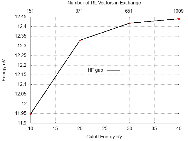
and looking at the column corresponding to Ehf value (column 4). For the number of G vectors corresponding to the cutoff energy cutoff in input search Exchange RL vectors in the report files. Note that it is not possible anymore to extract directly the HF gap from the report file as we did above, as in this case, we did not include all the BZ in the calculation. Now it possible to plot the energy gap in function of the energy cutoff or number of Gvectors:

$ gnuplot
gnuplot> plot "hf.dat" u 1:($4-$3)  w lp t "HF gap vs Energy cutoff"
gnuplot> plot "hf.dat" u 2:($4-$3)  w lp t "HF gap vs Number of G vector"

or you can plot the gap in function of both quantities using the hf.gnu gnuplot script:

and you can see that at 40Ry the energy gap is very close to convergence. Plotting the occupied and unoccupied bands separately you can recognize that for this system the unoccupied band does converge much faster.

The last important convergence test deals with the accuracy of the integral over the Brillouin zone in the expression of the Exchange Self-Energy, which translates into K point convergence. In order to test the K point sampling, you should:

1. perform a new non-scf calculation with a bigger k point grid,
2. convert wave functions and electronic structure to Yambo databases in a different directory as explained in the DFT and p2y module,
3. Initialize the Yambo databases,
4. Redo the steps explained in this section.

For now, however, you can skip this convergence test and continue the tutorial at How to obtain the quasiparticle band structure of a bulk material

Prev: GW

Now: Tutorials Home --> GW --> Hartree_Fock

Next: Back to GW