Real time Bethe-Salpeter Equation (TDSE): Difference between revisions
| Line 224: | Line 224: | ||
and then run the code. Notice the presence of the <code>COLL_SEX</code> among the options after <code>-J</code> | and then run the code. Notice the presence of the <code>COLL_SEX</code> among the options after <code>-J</code> | ||
yambo_rt -F Inputs_rt/04_td_hsex.in -J "TD- | nohup yambo_rt -F Inputs_rt/04_td_hsex.in -J "TD-SEX_rt,COLL_SEX" -C TD-SEX_rt | ||
and immediately after do the post processing | |||
ypp_rt -F Inputs/01_td_ip_ypp.in -J TD-sex_rt -C TD-SEX_rt | |||
=== Approach based on the Berry Phase === | === Approach based on the Berry Phase === | ||
| Line 232: | Line 235: | ||
yambo_nl -u -V qp -F Inputs_nl/04_td-sex.in | yambo_nl -u -V qp -F Inputs_nl/04_td-sex.in | ||
The input file is | |||
nloptics # [R NL] Non-linear optics | nloptics # [R NL] Non-linear optics | ||
| Line 269: | Line 273: | ||
Notice that in the calculation we decreased the number of G-vectors in the Hartree term, [[Variables#HARRLvcs|HARRLvcs]] to speed up the calculation, in case of BN this does not change the result because local field effects are very small in h-BN along the plane. | Notice that in the calculation we decreased the number of G-vectors in the Hartree term, [[Variables#HARRLvcs|HARRLvcs]] to speed up the calculation, in case of BN this does not change the result because local field effects are very small in h-BN along the plane. | ||
yambo_nl -F Inputs_nl/04_td_hsex.in -J "TD-SEX_nl,COLL_SEX" -C TD-SEX_nl | nohup yambo_nl -F Inputs_nl/04_td_hsex.in -J "TD-SEX_nl,COLL_SEX" -C TD-SEX_nl | ||
Now you can analyze the response with | Now you can analyze the response with | ||
Revision as of 15:49, 23 January 2020
Introduction
This tutorial will show how to perform a real-time calculation with Yambo on hBN monolayer. We will go through different approximations for the many body self--energy (HXC potential in the yambo language) up to the HSEX approximation which captures the physics of the exciton. For approximations local in space, like "TD-HARTREE" and "TD-DFT", the HXC potential can be evaluated directly during the simulation from real space quantities. On the contrary for approximations non local in space, one first need to compute the "real time collisions".
The same DFT inputs used to generate the hBN-2D-RT.tar.gz, are sufficient to converge the energy of the first exciton. You will need to increase the number of k-points to converge higher energy excitons.
TD Hartree and TD DFT
TD Hartree
yambo_rt -n p -v hartree -F Inputs_rt/02_td_hartree.in
 negf                           # [R] Real-Time dynamics
 HXC_Potential= "HARTREE"       # [SC] SC HXC Potential
 HARRLvcs= 1000        mHa      # [HA] Hartree RL components
 VXCRLvcs= 0.          mHa      # [HA] DFT     RL components
 % RTBands
   3 | 5 |                     # [RT] Bands
 %
 Integrator= "RK2"              # [RT] Integrator. Use keywords space separated  ( "EULER/EXPn/INV" "SIMPLE/RK2/RK4/HEUN" "RWA")
 PhLifeTime= 100.0000   fs      # [RT] Dephasing Time
 RTstep=10.000000       as      # [RT] Real Time step length
 NETime= 20.00000       fs      # [RT] Simulation Time
 % IOtime
  0.01     | 1.00     | 0.01     |  fs    # [RT] Time between to consecutive I/O (OBSERVABLEs,CARRIERs - GF - OUTPUT)
 %
 % Field1_Freq
  0.00     | 0.00     | eV      # [RT Field1] Frequency
 %
 Field1_Int= 1.E3   kWLm2   # [RT Field1] Intensity
 Field1_Width= 0.000000 fs      # [RT Field1] Width
 Field1_kind= "DELTA"            # [RT Field1] Kind(SIN|RES|ANTIRES|GAUSS|DELTA|QSSIN)
 Field1_pol= "linear"             # [RT Field1] Pol(linear|circular)
 % Field1_Dir
  0.000000 | 1.000000 | 0.000000 |        # [RT Field1] Versor
 %
 % Field1_Dir_circ
  0.000000 | 1.000000 | 0.000000 |        # [RT Field1] Versor_circ
 %
 Field1_Tstart= 0.000000fs      # [RT Field1] Initial Time
We set the cut-off on the Hartree potential to 1000 mHa. This defines the cutoff used to evaluate the Hartree potential at each time step. Notice also the need of setting the cutoff to Vxc to zero. This time we will propagate for just 20 fs. It is useful to run the simulation in background and then monitor the output file
 nohup yambo_rt -F ../Inputs_rt/02_td_hartree.in -J TD-HARTREE_1000mHa -C  TD-HARTREE_1000mHa &
 tail -f TD-HARTREE_1000mHa/o-TD-HARTREE_1000mHa.polarization
We can even have check the output on the fly.
To interrupt tail -f
ctrl+C
Then
 gnuplot
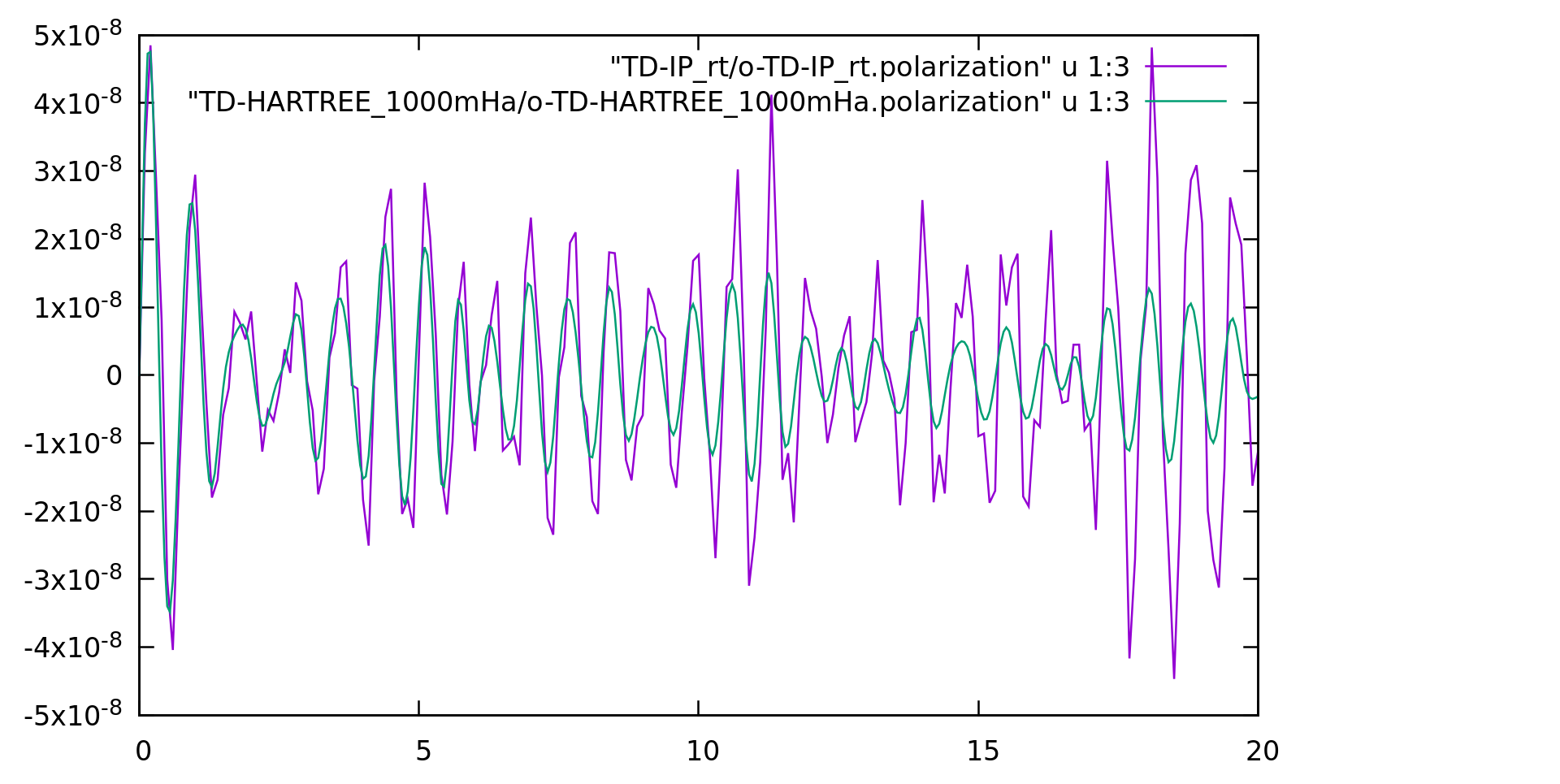
 plot "TD-IP_rt/o-TD-IP_rt.polarization" u 1:3 w l
 set xrange [0:20]
 rep "TD-HARTREE_1000mHa/o-TD-HARTREE_1000mHa.polarization" u 1:3 w l
We can already see from the output that the polarization is not very different from the IP one.
The major difference is indeed due to the presence of a damping (or dephasing term) in the output (PhLifeTime, i.e. the life-time of the phase).
If we check the timing of the simulation we see that most of the time is spent in the following subroutines:
                       el_density_matrix :    7.5074 s CPU (    4002 calls,    0.0019 s avg)
                               V_Hartree :    1.0405 s CPU (    4002 calls,    0.0003 s avg)
                       V_real_space_to_H :   23.8210 s CPU (  220220 calls,    0.0001 s avg)
                          RT Hamiltonian :   32.5007 s CPU (    4001 calls,    0.0081 s avg)
The evaluation of the Hartree potential by itself does not take too much time. It is more consuming to evaluate the real space density. However it is the projection of the potential into the transition space (V_real_space_to_H) which takes most of the time. RT_Hamiltonian is just (roughly) the sum of the two previous subroutines. You can see how these timings change if you increase the cutoff on the Hartree potential.
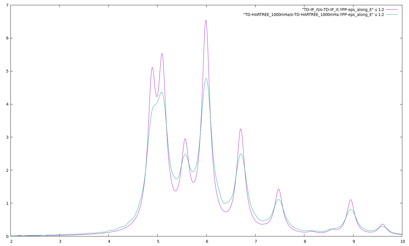
Thus we can expect that also the absorption will be quite similar. Indeed hBN is uniform in the plane.
As previously you can now to a post-processing of the polarization. The input file is exactly the same
 ypp_rt -F  Inputs_rt/01_td_ip_ypp.in -J TD-HARTREE_1000mHa -C TD-HARTREE_1000mHa
 gnuplot
 plot "TD-IP_rt/o-TD-IP_rt.YPP-eps_along_E" u 1:2 w l
 rep "TD-HARTREE_1000mHa/o-TD-HARTREE_1000mHa.YPP-eps_along_E" u 1:2 w l
 set xrange [2:10]
 rep
The situation would be completely different if we computed the polarization out of plane at both the TD-IP and the TD-Hartree level. You can try if you wish, but remember that you have to go back to the original SAVE folder and remove the symmetries not consistent with a field along the z direction this time: (see Prerequisites))
TD DFT
You can now try to perform a TDDFT simulation. Let's use the previous input file
cp Inputs_rt/02_td_hartree.in Inputs_rt/03_td_dft.in
and modify it
vim Input_rt/03_td_dft.in
 negf                            # [R] Real-Time dynamics
 HXC_Potential= "HARTREE+GS_XC"  # [SC] SC HXC Potential
 HARRLvcs= 1.E3       mHa        # [HA] Hartree     RL components
 VXCRLvcs= 1.E3       mHa
We can now run the TD-DFT simulation
 nohup yambo_rt -F Inputs_rt/03_td_dft.in -J TD-DFT_1000mHA -C TD-DFT_1000mHA &
 tail -f TD-DFT_1000mHA/o-TD-DFT_1000mHA.polarization
and once it is over do the post processing
 ctrl+C
 ypp_rt_4.5_gpl -F Inputs_rt/01_td_ip_ypp.in -J TD-DFT_1000mHA -C TD-DFT_1000mHA
 gnuplot
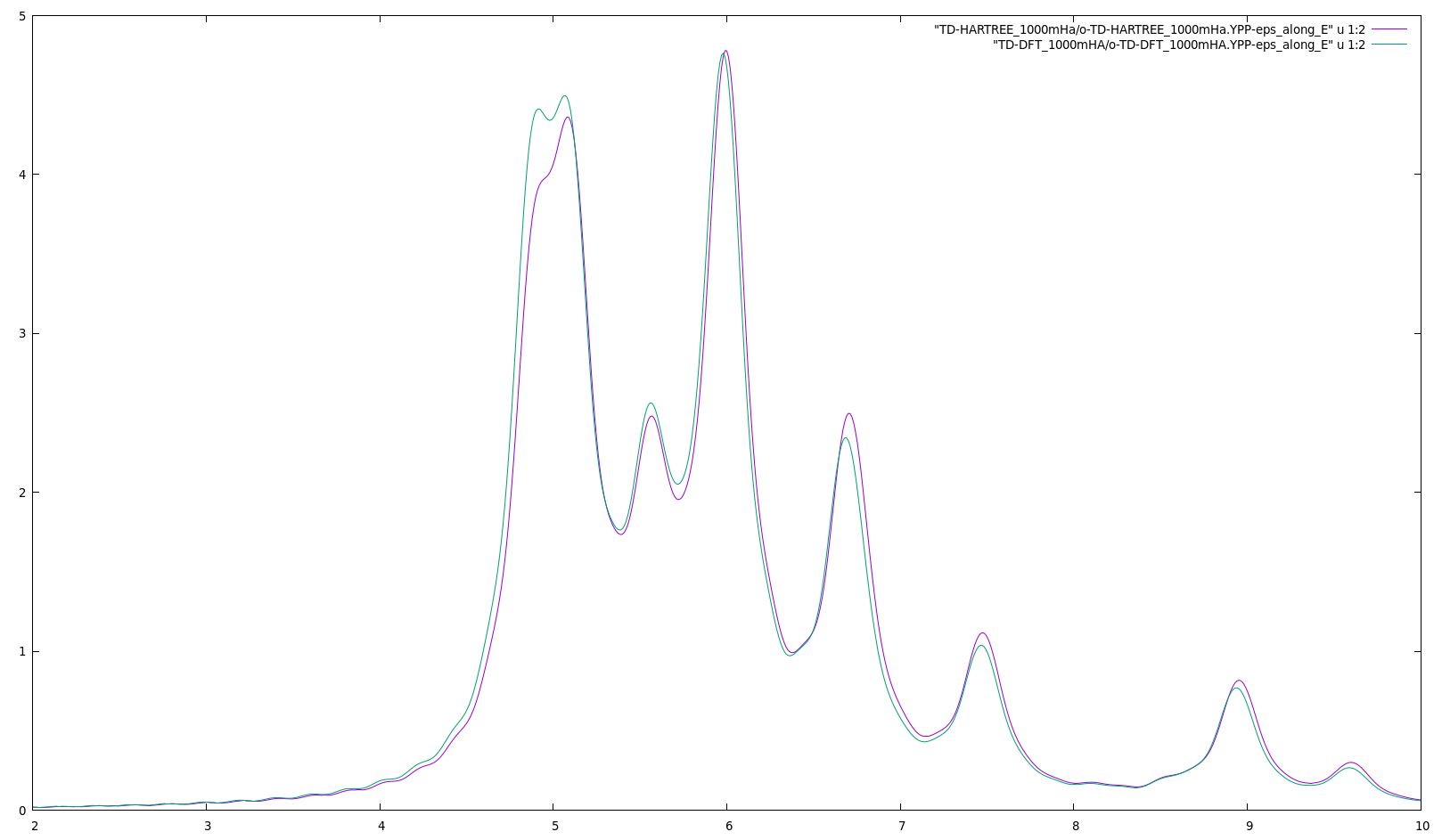
 gnuplot> plot "TD-HARTREE_1000mHa/o-TD-HARTREE_1000mHa.YPP-eps_along_E" u 1:2 w l
 gnuplot> rep "TD-DFT_1000mHA/o-TD-DFT_1000mHA.YPP-eps_along_E" u 1:2 w l
As expected TDDFT does not improve much over TD-HARTREE in extended systems
The Real Time Collisions
We next move to the evaluation of the collisions. (see Introduction to Real Time propagation in Yambo to remember what are the collisions)
This part is common in between the yambo_nl and the yambo_rt.
Then generate the input file to calculate the collisions (see appendix of Ref. [1]) use the command :
yambo_rt -b -e -v hsex -F Inputs_common/03_coll_hsex.in
The flag -b will tell the code to calculate the dielectric constant that is required for the screened interaction.
It could be even computed in an independent calculation and then loaded using the -J flags
em1s                           # [R Xs] Static Inverse Dielectric Matrix
dipoles                        # [R   ] Compute the dipoles
Chimod= "HARTREE"              # [X] IP/Hartree/ALDA/LRC/PF/BSfxc
% BndsRnXs
   1 |  20 |                   # [Xs] Polarization function bands
%
NGsBlkXs= 1000 mHa      # [Xs] Response block size
% DmRngeXs
  0.10000 |  0.10000 | eV      # [Xs] Damping range
%
% LongDrXs
 1.000000 | 0.000000 | 0.000000 |        # [Xs] [cc] Electric Field
%
While this is the part of the input file specific for the evaluation of the collisions
collisions                     # [R] Eval the extended Collisions
% COLLBands
  3 |  5  |                  # [COLL] Bands for the collisions
%
HXC_Potential= "HARTREE+SEX"           # [SC] SC HXC Potential
HARRLvcs= 1000 mHa      # [HA] Hartree     RL components
EXXRLvcs= 1000 mHa      # [XX] Exchange    RL components
CORRLvcs= 1000 mHa      # [GW] Correlation RL components
With this input, we calculate the HARTREE plus SEX collisions integrals. Notice that the HARTREE term in principle can be calculated on the fly, but in this way it is more efficient especially for the non-linear response.
Here one has to converge the cutoff for the Hartree and the Screened Exchange. Around 5000 mHa is a reasonable value for hBN. In this example we will use 1000 mHa to speed up calculations. The collisions bands COLLBands have to be the same number of bands you want to use in the linear/nonlinear response.
The you can run
yambo_rt -F Inputs_common/03_coll_hsex.in -J COLL_HSEX -C COLL_HSEX
The calculation will take about 1 minute in serial.
It produced many binary files ndb.COLLISIONS_HXC_fragment_* which will be needed to perform TD-HSEX simulations.
Notice that, if you want, you can also compute simple HARTREE collisions and use them in a TD-HARTREE simulation.
TD-HARTREE with collisions (facultative)
Then generate the input file to calculate the collisions (see appendix of Ref. [1]) use the command :
yambo_rt -e -v h -F Inputs_common/03_coll_hartree.in
with a simpler input file
collisions                     # [R] Eval the extended Collisions
% COLLBands
  3   |  5    |                 # [COLL] Bands for the collisions
%
HXC_Potential= "HARTREE"           # [SC] SC HXC Potential
HARRLvcs= 1000 mHa      # [HA] Hartree     RL components
 yambo_rt -F Inputs_common/03_coll_hartree.in -J COLL_HARTREE -C COLL_HARTREE
 yambo_rt -F Inputs_rt/02_td_hartree.in -J "TD-HARTREE_COLL,COLL_HARTREE" -C TD-HARTREE_COLL
and compare the run with the simulation without collision. One major difference, is that, when the collisions are used, yambo does not need to load the wave--function anymore and the simulation is much faster. The drawback is that for big systems the folder COLL_HARTREE may become huge, thus requiring a lot of disk space.
Time dependent Bethe Salpeter equation
Approach based on the density matrix
To generate the input for the real-time simulation you can run
yambo_rt -n p -v hsex -V qp -F Inputs_rt/04_td_hsex.in
As you can see this time the extra verbosity for quasi-particles is used -V qp
The reason is that, to be consistent with the TD-HSEX, simulation we need to apply quasi-particles corrections.
The input file is
 negf                           # [R] NEQ Real-time dynamics
 HXC_Potential= "SEX+HARTREE"   # [SC] SC HXC Potential
 % RTBands
   3 | 5 |                     # [RT] Bands
 %
 Integrator= "RK2"              # [RT] Integrator. Use keywords space separated  ( "EULER/EXPn/INV" "SIMPLE/RK2/RK4/HEUN" "RWA")
 PhLifeTime= 100.0000   fs      # [RT] Dephasing Time
 RTstep=10.000000       as      # [RT] Real Time step length
 NETime= 20.00000       fs      # [RT] Simulation Time
 % IOtime
  0.01     | 1.00     | 0.05     |  fs    # [RT] Time between to consecutive I/O (OBSERVABLEs,CARRIERs - GF - OUTPUT)
 %
 HARRLvcs= 1000       mHa      # [HA] Hartree     RL components
 EXXRLvcs= 1000       mHa      # [XX] Exchange    RL components
 CORRLvcs= 1000       mHa      # [GW] Correlation RL components
% GfnQP_E
 3.000000 | 1.000000 | 1.000000 |       # [EXTQP G] E parameters  (c/v) eV|adim|adim
%
 % Field1_Freq
  0.00     | 0.00     | eV      # [RT Field1] Frequency
 %
 Field1_Int= 1.E3   kWLm2   # [RT Field1] Intensity
 Field1_Width= 0.000000 fs      # [RT Field1] Width
 Field1_kind= "DELTA"            # [RT Field1] Kind(SIN|RES|ANTIRES|GAUSS|DELTA|QSSIN)
 Field1_pol= "linear"             # [RT Field1] Pol(linear|circular)
 % Field1_Dir
  0.000000 | 1.000000 | 0.000000 |        # [RT Field1] Versor
 %
 % Field1_Dir_circ
  0.000000 | 1.000000 | 0.000000 |        # [RT Field1] Versor_circ
 %
 Field1_Tstart= 0.000000fs      # [RT Field1] Initial Time
and then run the code. Notice the presence of the COLL_SEX among the options after -J
nohup yambo_rt -F Inputs_rt/04_td_hsex.in -J "TD-SEX_rt,COLL_SEX" -C TD-SEX_rt
and immediately after do the post processing
ypp_rt -F Inputs/01_td_ip_ypp.in -J TD-sex_rt -C TD-SEX_rt
Approach based on the Berry Phase
To generate the input for the real-time simulation you can run
yambo_nl -u -V qp -F Inputs_nl/04_td-sex.in
The input file is
nloptics                       # [R NL] Non-linear optics
DIP_Threads=0                  # [OPENMP/X] Number of threads for dipoles
NL_Threads=0                   # [OPENMP/NL] Number of threads for nl-optics
% NLBands
  4 |  5 |                     # [NL] Bands
%
NLverbosity= "low"             # [NL] Verbosity level (low | high)
NLstep=   0.0100       fs      # [NL] Real Time step length
NLtime= 55.00000       fs      # [NL] Simulation Time
NLintegrator= "CRANKNIC"         # [NL] Integrator ("EULEREXP/RK2/RK4/RK2EXP/HEUN/INVINT/CRANKNIC")
NLCorrelation= "SEX"           # [NL] Correlation ("IPA/HARTREE/TDDFT/LRC/LRW/JGM/SEX")
NLLrcAlpha= 0.000000           # [NL] Long Range Correction
% NLEnRange
 0.200000 | 8.000000 | eV      # [NL] Energy range
%
NLEnSteps= 1                   # [NL] Energy steps
NLDamping=  0.10000    eV      # [NL] Damping
#UseDipoles                    # [NL] Use Covariant Dipoles (just for test purpose)
#FrSndOrd                      # [NL] Force second order in Covariant Dipoles
#EvalCurrent                   # [NL] Evaluate the current
HARRLvcs= 1017         RL      # [HA] Hartree     RL components
EXXRLvcs= 1074         mHa     # [XX] Exchange    RL components
% ExtF_Dir
 0.000000 | 1.000000 | 0.000000 |        # [NL ExtF] Versor
%
ExtF_Int= 1000.        kWLm2   # [NL ExtF] Intensity
ExtF_Width= 0.000000   fs      # [NL ExtF] Field Width
ExtF_kind= "DELTA"             # [NL ExtF] Kind(SIN|SOFTSIN|RES|ANTIRES|GAUSS|DELTA|QSSIN)
ExtF_Tstart=   0.0100  fs      # [NL ExtF] Initial Time
% GfnQP_E
 3.000000 | 1.000000 | 1.000000 |        # [EXTQP G] E parameters  (c/v) eV|adim|adim
%
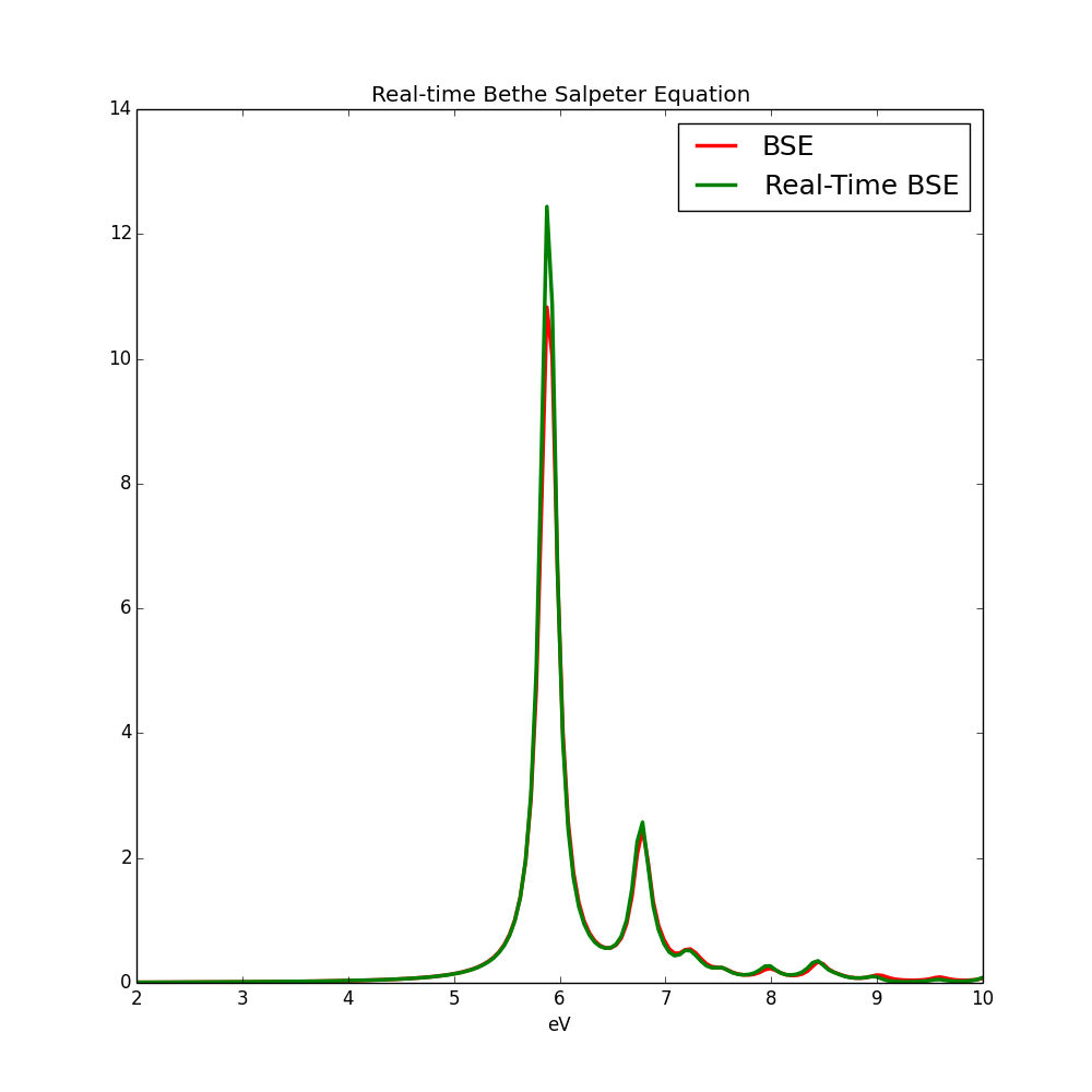
Notice that we introduced a scissor operator (a rigid shift of the conduction bands) of 3.0 eV. In principle, it is possible to perform a G0W0 calculation with Yambo and use the Quasi-particle band structure instead of the rigid shift. Run this calculation and then analyze the result in the same way of linear response tutorial, you will get a nice exciton in hBN, as the one plotted below in the old tutorial. You can repeat the same kind of calculations for the non-linear response. Notice that in the calculation we decreased the number of G-vectors in the Hartree term, HARRLvcs to speed up the calculation, in case of BN this does not change the result because local field effects are very small in h-BN along the plane.
nohup yambo_nl -F Inputs_nl/04_td_hsex.in -J "TD-SEX_nl,COLL_SEX" -C TD-SEX_nl
Now you can analyze the response with
ypp_nl -F Inputs_nl/01_ypp_nl.in -J TD-SEX_nl -C TD-SEX_nl
as it was done the linear response tutorial and compare with the standard Bethe-Salpeter (input here):
Linear response results can be obtained following the BSE tutorial. Notice that you can use the SEX approximation for the non-linear response too (see the following tutorials on non-linear response).
References
| Prev: Independent Particles | Now: ICTP Tutorials --> Linear Response --> Real time Bethe-Salpeter Equation (TDSE) | Next: If you did all steps you can go back to the previous level |


