GW tutorial. Convergence and approximations (BN): Difference between revisions
No edit summary |
No edit summary |
||
| Line 1: | Line 1: | ||
We have selected 2D hexagonal boron nitride to explain the use of yambopy. Along this tutorial we show how to use yambopy to make efficient convergence tests, to compare different approximations and to analyze the results. | We have selected 2D hexagonal boron nitride to explain the use of yambopy. Along with this tutorial we show how to use yambopy to make efficient convergence tests, to compare different approximations and to analyze the results. | ||
The initial step is to perform the ground state calculation and the non self-consistent calculation with Quantum Espresso using the <code>gs_bn.py</code> file: | The initial step is to perform the ground state calculation and the non self-consistent calculation with Quantum Espresso using the <code>gs_bn.py</code> file: | ||
| Line 62: | Line 62: | ||
analysebse -> Using ypp, you can study the convergence of BSE calculations in 2 ways: | analysebse -> Using ypp, you can study the convergence of BSE calculations in 2 ways: | ||
plotem1s -> Plot em1s calculation | plotem1s -> Plot em1s calculation | ||
analysegw -> Study the convergence of GW calculations by looking at the change in | analysegw -> Study the convergence of GW calculations by looking at the change in bandgap value. | ||
mergeqp -> Merge QP databases | mergeqp -> Merge QP databases | ||
test -> Run yambopy tests | test -> Run yambopy tests | ||
| Line 72: | Line 72: | ||
<source lang="python"> | <source lang="python"> | ||
Study the convergence of GW calculations by looking at the change in | Study the convergence of GW calculations by looking at the change in bandgap value. | ||
The script reads from <folder> all results from <variable> calculations and display them. | The script reads from <folder> all results from <variable> calculations and display them. | ||
| Line 94: | Line 94: | ||
</source> | </source> | ||
Running the function selecting the bands and | Running the function selecting the bands and k-points, together with the parameter of convergence we will obtain the convergence plot. | ||
<source lang="python">yambopy analysegw -bc 5 -kc 19 -bv 4 -kv 19 gw_conv EXXRLvcs | <source lang="python">yambopy analysegw -bc 5 -kc 19 -bv 4 -kv 19 gw_conv EXXRLvcs | ||
| Line 123: | Line 123: | ||
We will work in the PPA for the screening. We have chosen the following parameters: | We will work in the PPA for the screening. We have chosen the following parameters: | ||
<source lang="bash"> | <source lang="bash"> | ||
BndsRnXp = | EXXRLvcs = 80 Ry | ||
NGsBlkXp = | BndsRnXp = 25 bands | ||
GbndRnge = | NGsBlkXp = 3 Ry | ||
GbndRnge = 25 bands | |||
QPkrange = [1,19,2,6]</source> | QPkrange = [1,19,2,6]</source> | ||
We can just simply run the code to calculate the GW corrections for all the points of the Brillouin zone by setting the convergence parameters in the function gw of the script and doing: | We can just simply run the code to calculate the GW corrections for all the points of the Brillouin zone by setting the convergence parameters in the function gw of the script and doing: | ||
<source lang="bash">python gw_conv_bn.py -g</source> | <source lang="bash">python gw_conv_bn.py -g</source> | ||
The first image | The first image shows all the GW energies along all the k-points of the Brillouin zone. A clearer picture can be obtained by plotting the band structure along the symmetry points GMKG by using the analyser: | ||
<source lang="bash">python gw_conv_bn.py -r</source> | <source lang="bash">python gw_conv_bn.py -r</source> | ||
We first pack the results | We first pack the results into a json file and subsequently we use the analyser to create the object which contains all the information. | ||
<source lang="bash">pack_files_in_folder('gw') | <source lang="bash">pack_files_in_folder('gw') | ||
ya = YamboAnalyser('gw')</source> | ya = YamboAnalyser('gw')</source> | ||
The object <code>ya</code> contains all the results written in the output. We can plot any output variable. In yambopy we provide a function to plot the band structure along a given path. The BN band structure is shown below. The GW correction opens the LDA | The object <code>ya</code> contains all the results written in the output. We can plot any output variable. In yambopy we provide a function to plot the band structure along a given path. The BN band structure is shown below. The GW correction opens the LDA band gap as expected. | ||
[[File:GW-LDA-BN-bands.png|LDA (dashed lines) and GW (solid lines) band structures|500px]] | [[File:GW-LDA-BN-bands.png|LDA (dashed lines) and GW (solid lines) band structures|500px]] | ||
| Line 149: | Line 149: | ||
<source lang="bash">COHSEX | <source lang="bash">COHSEX | ||
BndsRnXs = 24 bands | BndsRnXs = 24 bands | ||
NGsBlkXs = | NGsBlkXs = 3 Ry | ||
PPA | PPA | ||
BndsRnXp = 24 bands | BndsRnXp = 24 bands | ||
NGsBlkXp = | NGsBlkXp = 3 Ry | ||
RA | RA | ||
BndsRnXd = 24 bands | BndsRnXd = 24 bands | ||
NGsBlkXd = | NGsBlkXd = 3 Ry</source> | ||
We have set the converged parameters and the function works by running: | We have set the converged parameters and the function works by running: | ||
| Line 168: | Line 168: | ||
=== Solvers (Newton, Secant, Green's function) === | === Solvers (Newton, Secant, Green's function) === | ||
The solvers to find the QP correction from the self-energy can also be tested. We have included the Newton and the secant method. In the resulting band structures we do not appreciate big differences. In | The solvers to find the QP correction from the self-energy can also be tested. We have included the Newton and the secant method. In the resulting band structures, we do not appreciate big differences. In any case it is worthy to test during the convergence procedure. | ||
[[File:GW-newton-secant.png|GW bands calculated with the methods Newton and Secant|500px]] | [[File:GW-newton-secant.png|GW bands calculated with the methods Newton and Secant|500px]] | ||
Revision as of 20:17, 27 April 2017
We have selected 2D hexagonal boron nitride to explain the use of yambopy. Along with this tutorial we show how to use yambopy to make efficient convergence tests, to compare different approximations and to analyze the results.
The initial step is to perform the ground state calculation and the non self-consistent calculation with Quantum Espresso using the gs_bn.py file:
<source lang="bash">python gs_bn.py
python gs_bn.py -sn</source>
We have set the non-self-consistent run with a wave-function cutoff of 60 Ry, 70 bands and a k-grid 12x12x1.
GW convergence
(a) Calculations
We converge the main parameters of a GW calculation independently. We make use of the plasmon pole approximation for the dielectric function and the Newton solver to find the GW correction to the LDA eigenvalues. The quantity to converge is the band gap of the BN (conduction and valence band at the K point of the Brillouin zone). We can select this calculation by calling the YamboIn with the right arguments:
<source lang="python">y = YamboIn('yambo -d -g n -p p -V all',folder='gw_conv')</source> The main variables are:
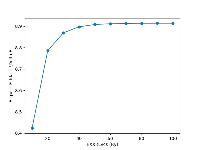
EXXRLvcs: Exchange self-energy cutoff
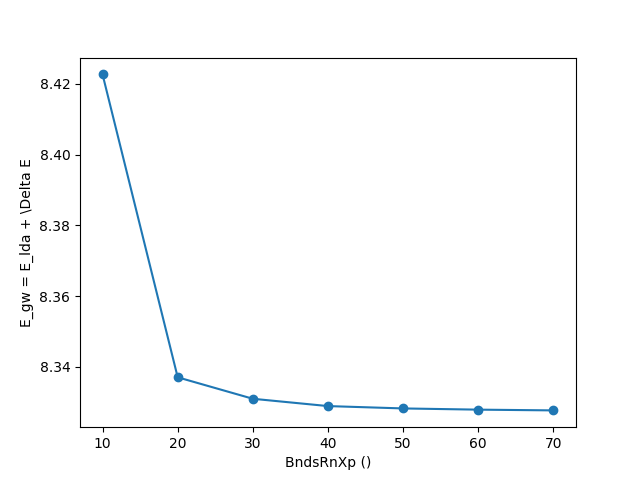
BndsRnXp: Number of bands in the calculation of the dielectric function (PPA).
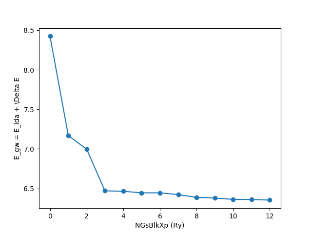
NGsBlkXp: Cutoff of the dielectric function.
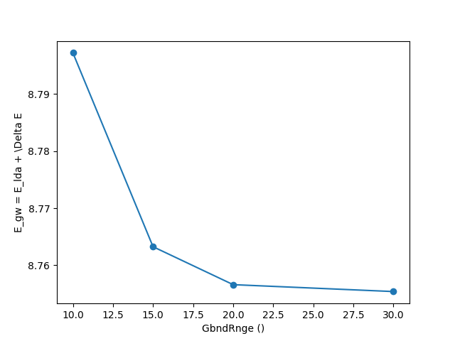
GbndRnge: Self-energy. Number of bands.
The convergence with the k-grid is done after these variables are converged and in principle is also independent of them. The convergence is set with a dictionary in which we choose the parameter and the values. Be aware of setting the right units and format for each parameter.
<source lang="python">conv = { 'EXXRLvcs': [[10,10,20,40,60,80,100],'Ry'],
        'NGsBlkXp': [[0,0,1,2,3,4], 'Ry'],
        'BndsRnXp': [[[1,10],[1,10],[1,20],[1,30]],] ,
        'GbndRnge': [[[1,10],[1,10],[1,20],[1,30]],] }</source>
The class YamboIn includes the function optimize, which is called here:
<source lang="python">y.optimize(conv,run=run,ref_run=False)</source> This optimization function just needs the convergence dictionary and the run instructions, given by the function:
<source lang="python">def run(filename):
   ""Function to be called by the optimize function ""
   folder = filename.split('.')[0]
   print(filename,folder)
   shell = bash()
   shell.add_command('cd gw_conv; %s -F %s -J %s -C %s 2> %s.log'%(yambo,filename,folder,folder,folder))
   shell.run()
   shell.clean()</source>
We set an interactive run, in the folder gw_conv. All the calculations will be made there with the corresponding jobname.
(b) Analysis
Once all the calculations are finished it's time to analyse them. Before we do that, let's look at the tools yambopy offers.
Yambopy uses the json format for posterior analysis of the results. To pack all the files in this format,
there is a recipe in yambopy to automatically perform this task on a folder:
<source lang="python"> pack_files_in_folder('gw_conv',save_folder='gw_conv') </source>
Besides the python module, yambopy can also be called in the terminal to perform some post-analysis tasks:
<source lang="python">
    $ yambopy
    analysebse ->     Using ypp, you can study the convergence of BSE calculations in 2 ways:
      plotem1s ->     Plot em1s calculation
     analysegw ->     Study the convergence of GW calculations by looking at the change in bandgap value.
       mergeqp ->     Merge QP databases
          test ->     Run yambopy tests
  plotexcitons ->     Plot excitons calculation
</source>
Calling yambopy analysegw will display the help of the function:
<source lang="python">
Study the convergence of GW calculations by looking at the change in bandgap value.
The script reads from <folder> all results from <variable> calculations and display them.
   Use the band and k-point options according to the size of your k-grid
   and the location of the band extrema.
       Mandatory arguments are:
           folder   -> Folder containing SAVE and convergence runs.
           var      -> Variable tested (e.g. FFTGvecs)
       Optional variables are:
           -bc, --bandc   (int)  -> Lowest conduction band number
           -kc, --kpointc (int)  -> k-point index for conduction band
           -bv, --bandv   (int)  -> Highest valence band number
           -kv, --kpointv (int)  -> k-point index for valence band
           -np, --nopack  (flag) -> Do not call 'pack_files_in_folder'
           -nt, --notext  (flag) -> Do not print a text file
           -nd, --nodraw  (flag) -> Do not draw (plot) the result
</source>
Running the function selecting the bands and k-points, together with the parameter of convergence we will obtain the convergence plot.
<source lang="python">yambopy analysegw -bc 5 -kc 19 -bv 4 -kv 19 gw_conv EXXRLvcs yambopy analysegw -bc 5 -kc 19 -bv 4 -kv 19 gw_conv NGsBlkXp yambopy analysegw -bc 5 -kc 19 -bv 4 -kv 19 gw_conv BndsRnXp yambopy analysegw -bc 5 -kc 19 -bv 4 -kv 19 gw_conv GbndRnge</source>
By calling python gw_conv_bn.py -p in the terminal, these steps will be performed automatically for this tutorial and you will see the plots below.
From the convergence plot we can choose now a set of parameters and repeat the calculation for finer k-grids until we reach convergence with the k-points. We have intentionally used non-converged parameters. Nevertheless, along this week you should have gotten enough expertise to push the convergence of the parameters and determine the correct convergence set of parameters. We invite you to enter in the python script, increase the parameters and check again the convergence for larger values!
GW calculation in a regular grid and plot in a path in the Brillouin zone
We will work in the PPA for the screening. We have chosen the following parameters:
<source lang="bash"> EXXRLvcs = 80 Ry BndsRnXp = 25 bands NGsBlkXp = 3 Ry GbndRnge = 25 bands QPkrange = [1,19,2,6]</source> We can just simply run the code to calculate the GW corrections for all the points of the Brillouin zone by setting the convergence parameters in the function gw of the script and doing:
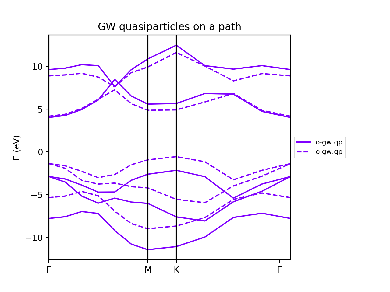
<source lang="bash">python gw_conv_bn.py -g</source> The first image shows all the GW energies along all the k-points of the Brillouin zone. A clearer picture can be obtained by plotting the band structure along the symmetry points GMKG by using the analyser:
<source lang="bash">python gw_conv_bn.py -r</source> We first pack the results into a json file and subsequently we use the analyser to create the object which contains all the information.
<source lang="bash">pack_files_in_folder('gw')
ya = YamboAnalyser('gw')</source>
The object ya contains all the results written in the output. We can plot any output variable. In yambopy we provide a function to plot the band structure along a given path. The BN band structure is shown below. The GW correction opens the LDA band gap as expected.
Approximations of the dielectric function (COHSEX, PPA, Real axis integration)
We can use yambopy to examine different run levels. For instance, the approximations used to obtain the screening are the: (i) static screening or COHSEX, plasmon-pole approximations (PPA), or real axis integration. We have set the same parameters for each run, just changing the variable name for the number of bands and the cut-off of the screening.
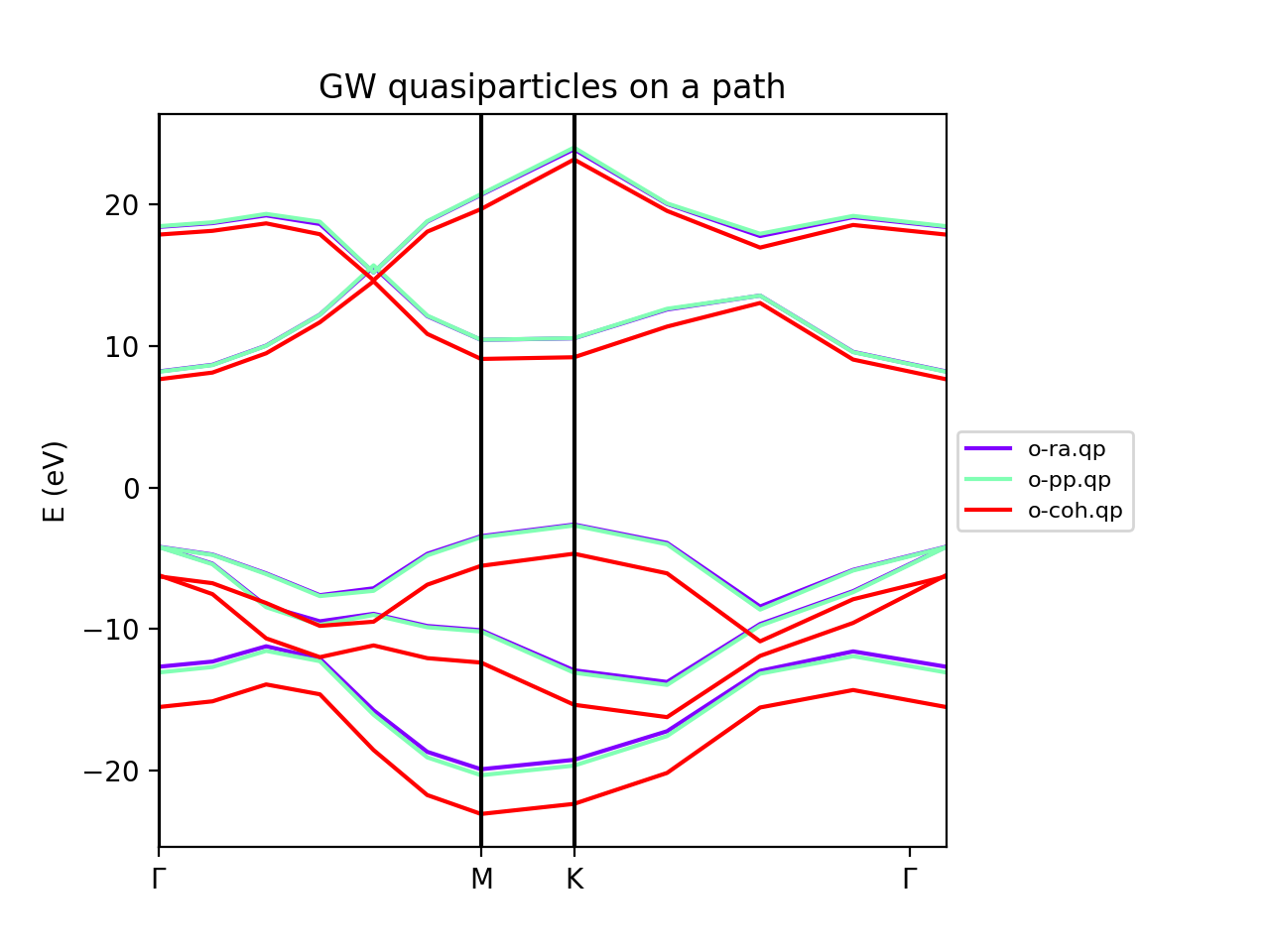
<source lang="bash">COHSEX BndsRnXs = 24 bands NGsBlkXs = 3 Ry PPA BndsRnXp = 24 bands NGsBlkXp = 3 Ry RA BndsRnXd = 24 bands NGsBlkXd = 3 Ry</source> We have set the converged parameters and the function works by running:
<source lang="bash">python gw_conv_bn.py -x</source> We plot the band structure using the analyzer explained above.
<source lang="bash">python gw_conv_bn.py -xp</source> The PPA and the RA results are basically on top of each other. On the contrary, the COHSEX (static screening) makes a poor job, overestimating the bandgap correction.
Solvers (Newton, Secant, Green's function)
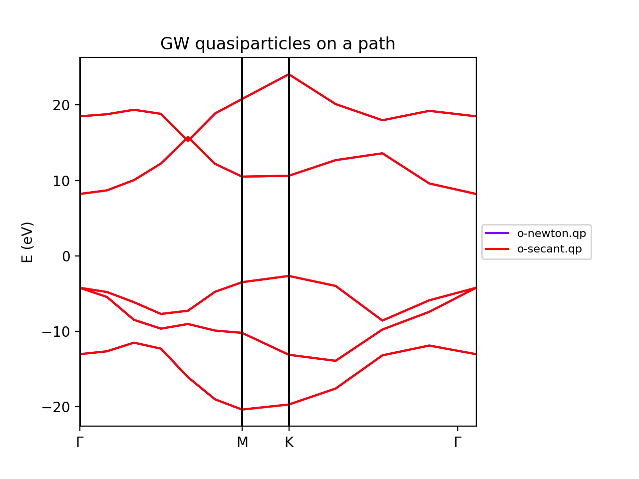
The solvers to find the QP correction from the self-energy can also be tested. We have included the Newton and the secant method. In the resulting band structures, we do not appreciate big differences. In any case it is worthy to test during the convergence procedure.
