Pushing convergence in parallel: Difference between revisions
(→2D hBN) |
(→2D hBN) |
||
| Line 7: | Line 7: | ||
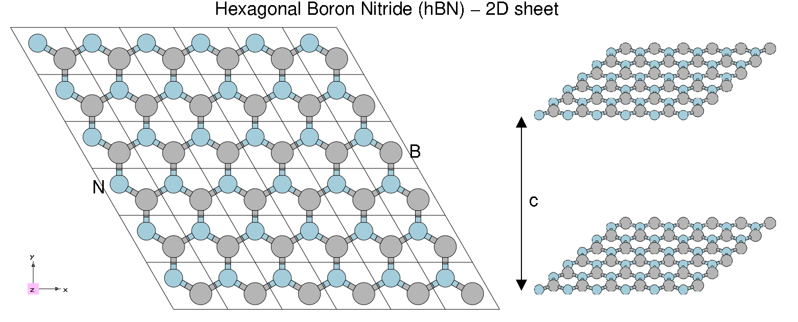
[[File:HBN2.png|500px|center|Atomic structure of 2D hBN]] | [[File:HBN2.png|500px|center|Atomic structure of 2D hBN]] | ||
If you | If you want a published reference of quasi-particle properties of hBN you can have a look to the following arxiv, | ||
https://arxiv.org/abs/1511.00129 (Phys. Rev. B 94, 155406 (2016)) | https://arxiv.org/abs/1511.00129 (Phys. Rev. B 94, 155406 (2016)), | ||
and references therein were the | and references therein, were the GW correction are computed. | ||
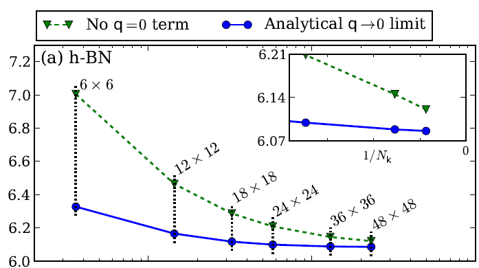
In that case the convergence with the number of k-points is studied in detail (for hBN and other materials). | In that case the convergence with the number of k-points is studied in detail (for hBN and other materials). | ||
The focus is on a proper description of the q->0 limit of the (screened) electron-electron | The focus is on a proper description of the q->0 limit of the (screened) electron-electron | ||
interaction entering the GW self-energy. | interaction entering the GW self-energy. | ||
As you can see from the below image extracted from the arxiv the QP corrections converge slowly with the number of k-points. | |||
[[File:QP convergence hBN from literature.png|400px|center|Yambo tutorial image]] | [[File:QP convergence hBN from literature.png|400px|center|Yambo tutorial image]] | ||
In the present tutorial you will start using a 12x12 grid. | In the present tutorial you will start using a 12x12 grid. | ||
Only in the last part we will re-run pw.x to generate bigger k-grids | Only in the last part we will re-run pw.x (optional) to generate bigger k-grids | ||
Tomorrow you will learn how to do that in a more automatic way using the yambopy scripting tools, however running yambo in serial. | |||
Tomorrow you will learn how to do that in a more automatic way using the yambopy scripting tools, | |||
however running yambo in serial. | |||
While yambopy offers an easier interface for the use, in the present parallel tutorial you | While yambopy offers an easier interface for the use, in the present parallel tutorial you | ||
will be able to push much more the convergence. In a real life calculation you will likely take advantage | will be able to push much more the convergence. In a real life calculation you will likely take advantage | ||
Revision as of 07:42, 26 April 2017
2D hBN
In the previous session we focused on the scaling properties of the code. We now focus more on the physical aspect.
The system we are working on is the 2D-hBN sheet we already used the first day.
If you want a published reference of quasi-particle properties of hBN you can have a look to the following arxiv, https://arxiv.org/abs/1511.00129 (Phys. Rev. B 94, 155406 (2016)), and references therein, were the GW correction are computed. In that case the convergence with the number of k-points is studied in detail (for hBN and other materials). The focus is on a proper description of the q->0 limit of the (screened) electron-electron interaction entering the GW self-energy. As you can see from the below image extracted from the arxiv the QP corrections converge slowly with the number of k-points.
In the present tutorial you will start using a 12x12 grid. Only in the last part we will re-run pw.x (optional) to generate bigger k-grids
Tomorrow you will learn how to do that in a more automatic way using the yambopy scripting tools, however running yambo in serial. While yambopy offers an easier interface for the use, in the present parallel tutorial you will be able to push much more the convergence. In a real life calculation you will likely take advantage of both.
Convergence on the number bands in X and G
Run changing the input parameters as follow:
The you can use the parse_qp.py script to extract the direct gap using the command
./parse_qp.py $jobname/o-*.qp
The output should be something similar to
#nbnd ibndval  Egap [eV]
  25    4        6.848440000
  50    4        6.759580000
  75    4        6.724210000
 100    4        6.712120000
 200    4        6.717220000
 400    4        6.733410000
Convergence with the energy cut-off on the response function
Convergence with the number of k-points (optional)
| Prev: Tutorials Home | Now: Tutorials Home --> GW Convergence | Next: Parallel tutorials are over |

