How to analyse excitons

In this tutorial you will learn (for a 2D-hBN) how to:

• How to analyze a BSE optical spectrum in terms of excitonic eigenvectors and eigenvalues
• How to plot the excitonic wavefunction

Prerequisites

Previous modules

• You must have completed the tutorial on 2D hBN.
• You must have completed the tutorial on 2D hBN.

You will need:

• ypp executable
• xcrysden executable
• gnuplot or xmgrace executable

YAMBO calculations

If you have completed the tutorials of 2D hBN you should have all the databases required to do this tutorial in your SAVE and 2D directories

$ ls ./SAVE
ndb.gops ndb.kindx ns.db1  ns.kb_pp_pwscf_fragment_1 ....
$ ls ./2D

ndb.BS_Q1_CPU_0 ndb.cutoff ndb.dip_iR_and_P_fragment_1 ndb.pp_fragment_1 ...

Sorting the excitonic eigenvalues

$ ypp -e -s -J 2D 

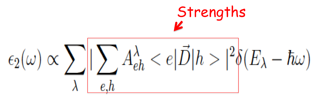
The new generated file o-2D.exc_E_sorted (o-2D.exc_E_sorted) reports the energies of the excitons and their Dipole Oscillator Strenghts sorted by energy (Index).

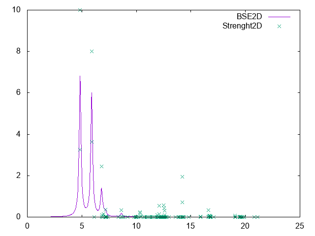
Open the first file and look inside. The first exciton is at 4.83 eV and the second one has the highest strenght (normalized to 1) Attention: clearly the convergence of these results has to be checked doing several BSE calculations with different k-grids!

Or you can make a plot

$ gnuplot
gnuplot> plot 'o-2D.eps_q1_diago_bse' w l title 'BSE2D' ,'o-2D.exc_E_sorted' u 1:($2*10) title 'Strenght2D'

Analyze the excitons

We can now analyze the excitons in terms of single-particle states to do that create the appropriate input

$ ypp -e a -F ypp.AMPL.in -J 2D

To analyze the first 5 excitons change this line as:

States= "1 - 5"              # Index of the BS state(s)

Close the input and run ypp

$ ypp -J 2D -F ypp_AMPL.in

$ls ls o*exc*at*
o-2D.exc_amplitude_at_1 o-2D.exc_weights_at_1 ...

Open the files for the first exciton: o-2D.exc_weights_at_1 reports the Weights, while o-2D.exc_weights_at_1 the amplitudes.

For an exciton [math]\displaystyle{ |\lambda\gt }[/math], the weights are defined as

and the amplitudes are defined as