Modena 2025 : Yambopy part 1

The first section of this tutorial will show you how to visualise wave-function and band-structure related information, such as atomic, orbital and spin projections, following a DFT Quantum Espresso calculation using the "qepy" submodule of Yambopy. In the second section, we will start using the "yambopy" submodule to read the Yambo binary databases in order access reciprocal space data, dipole matrix elements and the RPA response function.

In order to run both parts 1 and 2, you need to copy and extract the tar file named yambopy_tutorial_Modena_2025.tar.gz that you find in the WORK directory:

cd $SCRATCH
mkdir YAMBOPY_TUTORIALS
cd YAMBOPY_TUTORIALS
rsync -avzP /leonardo_work/tra25_yambo/YAMBOPY_TUTORIALS/yambopy_tutorial_Modena_2025.tar.gz .
tar -xvzf yambopy_tutorial_Modena_2025.tar.gz

Plot band structures from Quantum ESPRESSO

Tutorial 1. BN (semiconductor). Band structure

First enter in the folder

cd databases_qepy/bn-semiconductor

and have a look to the

vim plot-qe-bands.py

The qepy classes are useful both to execute Quantum Espresso and to analyze the results. Enter in the python environment, by typing python, then the full qepy library is imported by simply doing:

from qepy import *

Plot Band structure

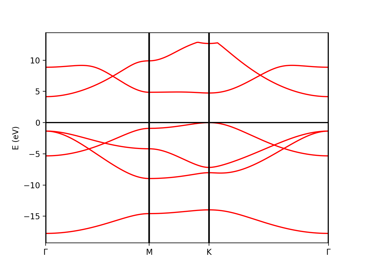
The qepy class PwXML reads the data file generated by Quantum Espresso and post-processes the data. The class is instanced by doing:

xml = PwXML(prefix='bn', path='bands')

The variable prefix corresponds to the same variable of the QE input. The folder location is indicated by variable path. In order to plot the bands, we also define the k-points path (in crystal coordinates) using the function Path:

npoints = 50
path_kpoints = Path([ [[0.0, 0.0, 0.0],'$\Gamma$'],
                      [[0.5, 0.0, 0.0],'M'],
                      [[1./3,1./3,0.0],'K'],
                      [[0.0, 0.0, 0.0],'$\Gamma$']], [int(npoints*2),int(npoints),int(sqrt(5)*npoints)])

It is worth to note that the path should coincide with the selected path for the QE band calculations.

In order to show the plot we can call the plot_eigen method of the PwXML class:

xml.plot_eigen(path_kpoints)

This function will automatically plot the bands. Alternatively, we can use the function plot_eigen_ax:

fig = plt.figure()
ax = fig.add_subplot(1,1,1)
xml.plot_eigen_ax(ax,path_kpoints)

This functions requires as input a matplotlib figure object with given axes. We can produce a figure by running the script:

python plot-qe-bands.py

Plot atomic orbital projected Band structure

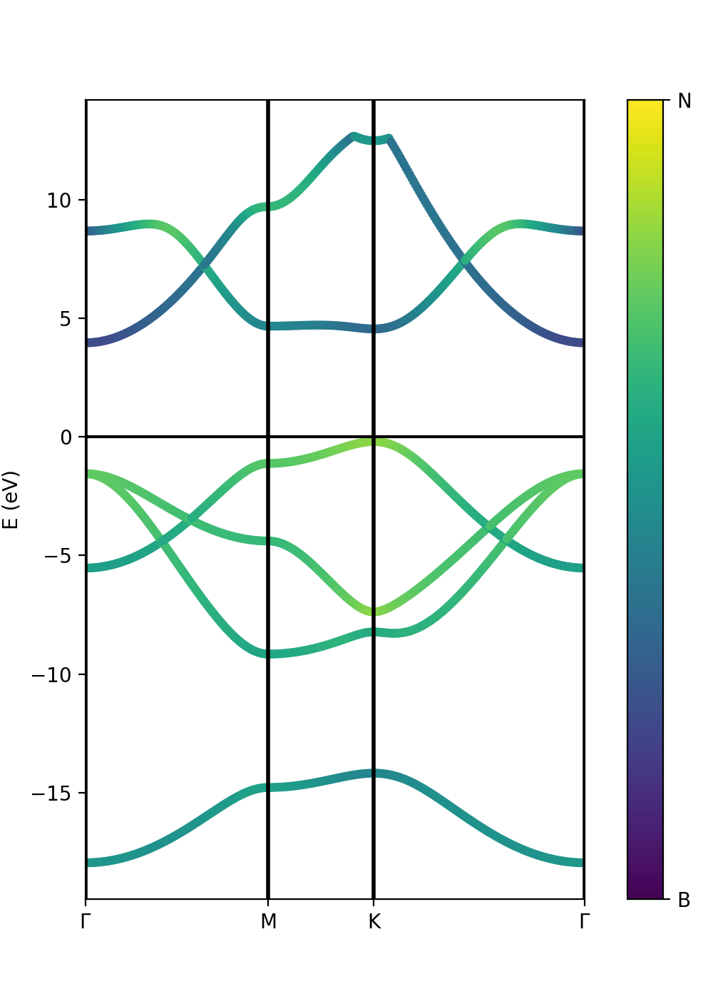
In addition to the band structure, useful information regarding the atomic orbital nature of the electronic wave functions can be displayed using the class ProjwfcXML. In order to make quantum espresso calculate the relevant data, we need to use the QE executable projwfc.x, which will create the file atomic_proj.xml. This executable projects the Kohn-Sham wavefunctions onto orthogonalized atomic orbitals, among others functionalities. The orbital indexing and ordering are explained in the input documentation of the projwfc.x function which you are invited to check (https://www.quantum-espresso.org/Doc/INPUT_PROJWFC.html#idm94). In this example, projwfc.x has been already run.

As in the class PwXML, we then define the path_kpoints and also the selected atomic orbitals to project our bands. We have chosen to represent the projection weight onto the nitrogen (1) and boron (2) orbitals, which can be obtained with

# Automatic selection of the states
atom_1 = band.get_states_helper(atom_query=['N'])
atom_2 = band.get_states_helper(atom_query=['B'])

The full list of orbitals is written in the file bands/prowfc.log. By inspecting it, you may also construct custom lists of states.

We have also defined the figure box

import matplotlib.pyplot as plt
fig = plt.figure(figsize=(5,7))
ax  = fig.add_axes( [ 0.12, 0.10, 0.70, 0.80 ])

The class ProjwfcXML then runs as in this example:

band = ProjwfcXML(prefix='bn',path='bands',qe_version='7.0')
band.plot_eigen(ax,path_kpoints=path_kpoints,cmap='viridis',selected_orbitals=atom_1,selected_orbitals_2=atom_2)

We can run now the file:

python plot-qe-orbitals.py

We have chosen the colormap 'viridis' (variable cmap). You see that the colormap goes from maximum selected_orbitals content (in this case nitrogen) to the maximum selected_orbitals_2 content (in this case boron). The colormap can be represented in many ways and qepy does not include a particular function for this. An example is:

import matplotlib as mpl
cmap=plt.get_cmap('viridis')
bx  = fig.add_axes( [ 0.88, 0.10, 0.05, 0.80 ])
norm = mpl.colors.Normalize(vmin=0.,vmax=1.)
cb1 = mpl.colorbar.ColorbarBase(bx, cmap=cmap, norm=norm,orientation='vertical',ticks=[0,1])
cb1.set_ticklabels(['B', 'N'])

Suppose now that we have run a G0W0 calculation (see part 2 of the Yambopy tutorial), and we want to represent the atomic weights on top of the quasiparticle band structure instead of the Kohn-Sham one. However, we do not have the same kpoint grid between the G0W0 calculation and the quantum espresso "band" calculation along a path. We can then extract the parameters for a scissor operator (this is done in part 2) and feed them to the ProjwfcXML class together with the number of valence bands. Try uncommenting the following lines in the tutorial script:

# Add scissor operator to the bands from a G0W0 calculation
scissor= [1.8985195950522469, 1.0265240811345133, 1.051588659878575]
n_val = 4
band.add_scissor(n_val,scissor)
 

Finally, we can also plot the band orbital character with size variation instead of a color scale. In this case we have to pass only the variable selected_orbitals (see below).

Tutorial 2. Iron. Ferromagnetic metallic material

Let's move to a magnetic system:

cd ../iron-metal

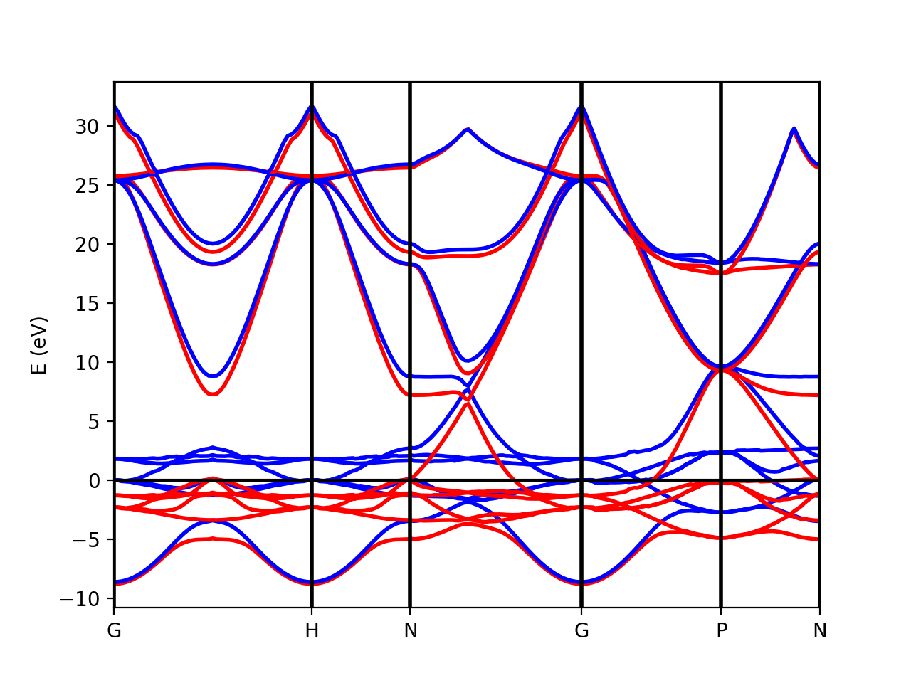
In the case of spin-polarized calculations we can plot the spin up and down band structures. After completing a band structure calculation for iron with Quantum ESPRESSO, we can make the band plot by running the script:

python plot-qe-bands.py

The class PwXML automatically detects the spin polarized case (nspin=2 in the QE input file). The spin up channel is displayed with red and the spin down channel with blue. In the case of iron we have selected this k-point path:

npoints = 50
path_kpoints = Path([ [[0.0, 0.0, 0.0 ],'G'],
                      [[0.0, 0.0, 1.0 ],'H'],
                      [[1./2,0.0,1./2.],'N'],
                      [[0.0, 0.0, 0.0 ],'G'],
                      [[1./2, 1./2, 1./2 ],'P'],
                      [[1./2,0.0,1./2. ],'N']], [npoints,npoints,npoints,npoints,npoints])

xml = PwXML(prefix='pw',path='bands/t0')
#xml.plot_eigen(path_kpoints)
fig = plt.figure()
ax = fig.add_subplot(1,1,1)
xml.plot_eigen_ax(ax,path_kpoints,lw=1.5)

The analysis of the projected atomic orbitals is also implemented. In this case the results are more cumbersome because the projection is separated in spin up and down channels.
Let us look first at the file plot-qe-orbitals-size.

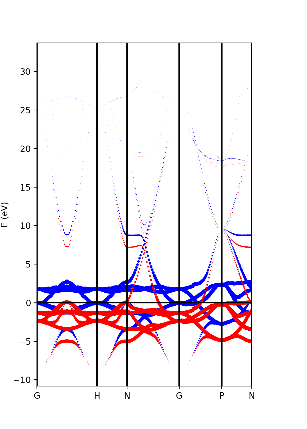
We can use the dot size as a function of the weight of the orbitals

# Automatic selection of the states
s = band.get_states_helper(orbital_query=['s'])
p = band.get_states_helper(orbital_query=['p'])
d = band.get_states_helper(orbital_query=['d'])

and the plots are done with

band = ProjwfcXML(prefix='pw',path='bands/t0',qe_version='7.0')
band.plot_eigen(ax,path_kpoints=path_kpoints,selected_orbitals=s,color='pink',color_2='black')
band.plot_eigen(ax,path_kpoints=path_kpoints,selected_orbitals=p,color='green',color_2='orange')
band.plot_eigen(ax,path_kpoints=path_kpoints,selected_orbitals=d,color='red',color_2='blue')

As an example, we can select just the d orbitals by commenting the first two plots and then running the file:

plot-qe-orbitals-size.py

From the plot is clear that d orbitals are mainly localized around the Fermi energy. The plot above is in red and blue, while the default choice in your script should be pink and black. You can experiment with the colors and other matplotlib plot options and also plot the other orbital types.

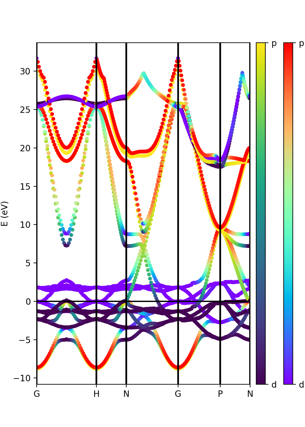
Another option is to plot the orbital composition as a colormap running the file:

plot-qe-orbitals-colormap.py

Here we have added the p and d orbitals in the analysis:

p = band.get_states_helper(orbital_query=['p'])
d = band.get_states_helper(orbital_query=['d'])
band = ProjwfcXML(prefix='pw',path='bands/t0',qe_version='7.0')
band.plot_eigen(ax,path_kpoints=path_kpoints,cmap='viridis',cmap2='rainbow',selected_orbitals=p,selected_orbitals_2=d)

The colormap bar is added in the same way as in Tutorial 1 (see script), but this time we have a different colormap for each spin polarisation.

YAMBO: deal with the databases

Let us now move to the directory containing some precalculated yambo databases:

cd ../../databases_yambopy

Tutorial 3: generating the Yambo SAVE via command line

Yambopy offers a set of command line options. In order to review them, you can type

yambopy

which will print the output

yambopy v0.4
Available commands are:

       plotem1s ->     Plot em1s calculation
     analysebse ->     Using ypp, you can study the convergence of BSE calculations in 2 ways:
      analysegw ->     Study the convergence of GW calculations by looking at the change in band-gap value.
   plotexcitons ->     Plot excitons calculation
          addqp ->     Add corrections from QP databases.
        mergeqp ->     Merge QP databases
           save ->     Produce a SAVE folder
           gkkp ->     Produce a SAVE folder including elph_gkkp databases
          bands ->     Script to produce band structure data and visualization from QE.
         serial ->     Script to update serial numbers of yambo ndb.* databases in order to import them to new calculations.
     gwsubspace ->     Script to calculate off-diago corrections of yambo ndb.QP databases in order to plot band structure.
          phinp ->     Script to update the explicit list of q-points in a ph input file (ldisp=.false., qplot=.true.).
        convert ->     Script to convert RL number in Ry energy units using ndb.gops.
        bsesize ->     Script to calculate the expected BSE kernel size, in GB, to be loaded by each MPI task
            l2y -> 	Calculate gauge-invariant electron-phonon matrix elements with LetzElPhC and convert them into Yambo format
           test ->     Run yambopy tests

By typing in one of the options, additional information about how to run the commands will be printed, e.g.:

yambopy save

Produce a SAVE folder

Arguments are:
  -nscf, --nscf_dir  -> Path to nscf save folder
  -y, --yambo_dir    -> <Optional> Path to yambo executables

Remember to load the yambo module, so that yambopy has access to the p2y and yambo executables. The quantum espresso save for hBN is provided in the directory BSE_saves/QE_saves/hBN.save (you can check the contents of the various folders). Then, following the instructions printed on screen, we can generate a yambo SAVE from the hBN.save by typing

yambopy save -nscf BSE_saves/QE_saves/hBN.save

This should produce a SAVE folder in the current directory.

Tutorial 4: Lattice intro (plot k-point coordinates in IBZ/BZ)

For this section we will use the script bz_plot.py.

By inspecting the SAVE folder we have just generated, we will find the ns.db1 database which contains all the geometry and lattice information. We are now going to read it in python by using the Yambopy class YamboLatticeDB, which can be instanced like this:

from yambopy import YamboLatticeDB
ylat = YamboLatticeDB.from_db_file(filename="PATH/TO/SAVE/ns.db1")

(remember to edit the variable save_path in order to point at your yambo SAVE).

The ylat object now contains many useful information as attributes, such as the k-points in Cartesian or crystal coordinates, the system symmetries, lattice constants and basis vectors in real and reciprocal space, etc. The k-points are also automatically expanded in the full Brillouin zone from the irreducible one (you can turn this off with the option Expand=False).

Directly printing the object with

print(ylat)

will also give us some general parameters related to the database.

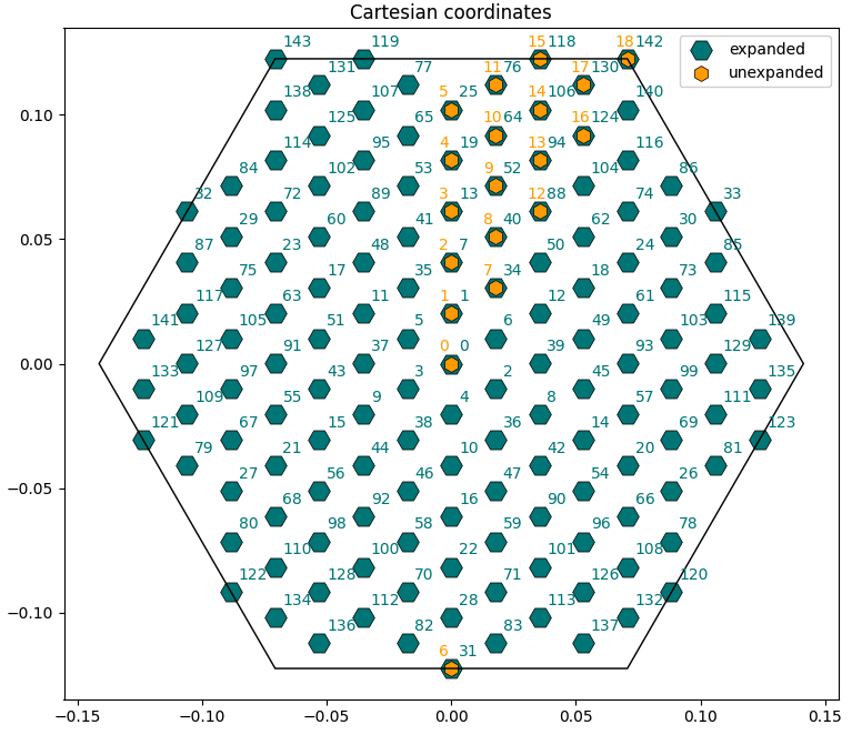
Now check the bz_plot.py script. You will see that it performs three plots:

• Scatterplot of the k-points in Cartesian coordinates with both expanded and unexpanded grids, with annotated indices [Cartesian_Plot=True].
• Scatterplot of the k-points in crystal coordinates [Crystal_Plot=True].
• Manual transformation of a chosen k-point from irreducible to full Brillouin zone (you can change the index i_k in the script to check different cases) [Symmetry_Plot=True].

Dipoles intro: plots of dipoles on BZ, plot of IP absorption

In this section we will use the script dipoles_plot.py and read the dipole databases generated in an optical absorption calculation by yambo. Keep in mind that from now on we will use the "BSE" yambo SAVE generated in the first section.

The databases written after a calculation of optical properties with yambo (dipoles, static screening, excitons) are in the directory BSE_saves/BSE_databases. Here we will also find ndb.dipoles which is needed now, since it contains the matrix elements d_{vck}(\alpha) where vk and ck are the valence and electron states involved in the transition and \alpha the polarisation direction of the external electric field.

In order to read it in python we use the Yambopy class YamboDipolesDB, which can be instanced like this:

ydip = YamboDipolesDB(ylat,save='path/to/BSE/databases',filename='ndb.dipoles')

(notice that it requires a previous instance of YamboLatticeDB).

In addition, in order to read the Kohn-Sham energies, we can also instance the YamboElectronsDB as

yel = YamboElectronsDB.from_db_file(folder='path/to/SAVE') 

The object ydip now has a method that permits to retrieve the independent-particle absorption spectrum with customly chosen energy range, steps, and broadening:

w, eps2 = ydip.ip_eps2(yel)

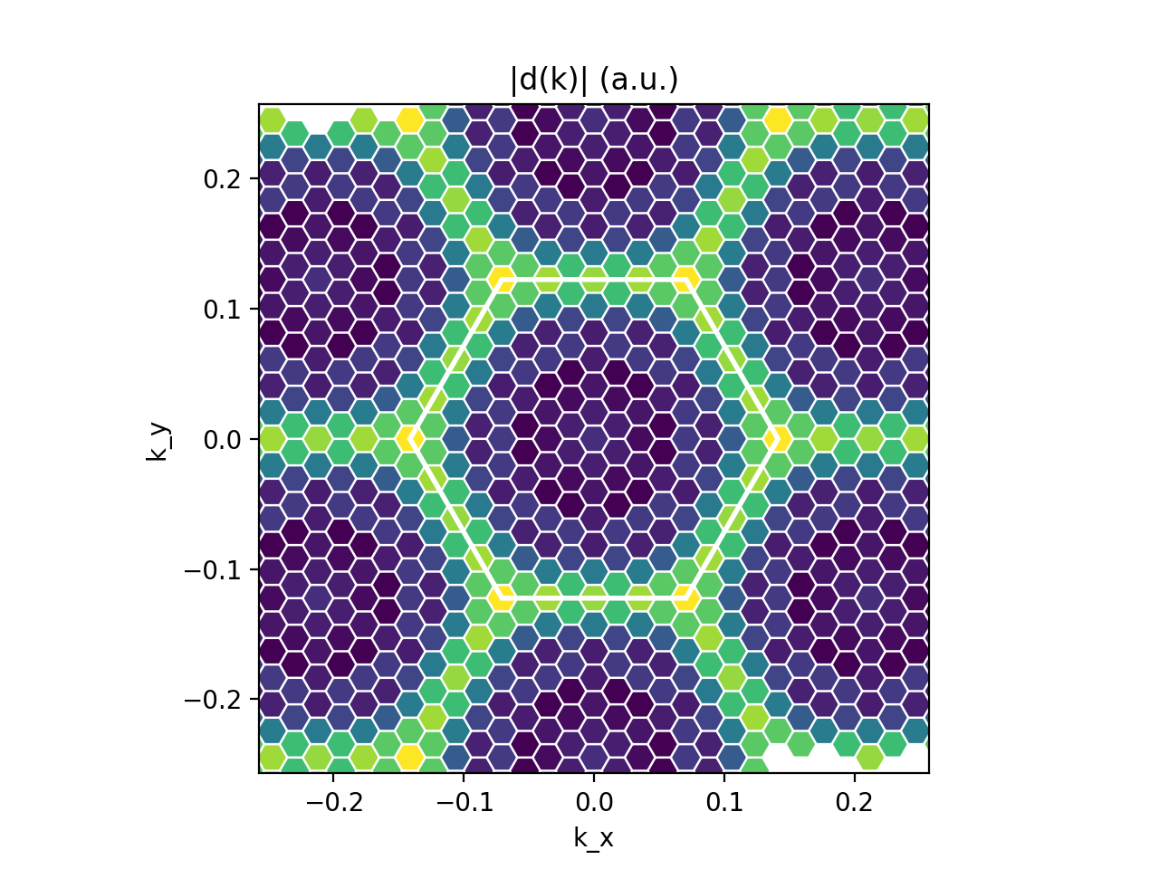
In order to see all this in action, take a look at the dipoles_plot.py script. You will see that it performs two plots:

• Plot of |d(k)| in the BZ for selected v,c and \alpha (we choose the layer plane 'xy') [Kspace_Plot=True]. From this plot you can appreciate which sections of the BZ contribute the most to the absorption rate.
• Plot of the independent-particles absorption spectrum [Absorption_Plot=True].

You can play with the indices and the plot parameters to check what happens.

Links

• Back to Modena 2025