Pump and Probe

This tutorial works only with Yambo version > 5.1, that will be released soon.

In this tutorial we will show you how to setup two external fields in yambo_nl, to perform pump and probe simulation.
This tutorial is at independent particle level, but the same kind of simulation can be repeated including local field effects, quasi-particle correction or electron-hole interaction, see for example the tutorials:

Correlation effects in the non-linear response
Real time Bethe-Salpeter Equation (TDSE)

This tutorial supposes that you are already familiar with real-time simulation with Yambo, if it is not the case please check these tutorials: Tutorials#Non_linear_response

We start from the h-BN monolayer with an in place lattice constant a=2.5 Å and a box large 30 a.u. in the z-direction. Standard DFT input for hBN monolayer for ABINIT or QuantumEspresso can be found here Tutorials.
We used a 9x9x1 k-points grid and 8 bands in the non-self consistent calculation. In order to have faster calculation we advice you to decrease the k-points grid to 12x12x1, results will be very close to the converged ones.

In our example we choose direction [0,1,0] for the pump and directions [1,0,0] e [0,1,0] for the probe. We generate the ypp.in to remove symmetries with the command ypp -y and we modify it as:

fixsyms                          # [R] Remove symmetries not consistent with an external perturbation
% Efield1
 0.000000 | 1.000000 | 0.000000 |        # First external Electric Field
%
% Efield2
 1.000000 | 0.000000 | 0.000000 |        # Additional external Electric Field
%
BField= 0.000000           T     # [MAG] Magnetic field modulus
Bpsi= 0.000000             deg   # [MAG] Magnetic field psi angle [degree]
Btheta= 0.000000           deg   # [MAG] Magnetic field theta angle [degree]
#RmAllSymm                     # Remove all symmetries 
RmTimeRev                     # Remove Time Reversal
#RmSpaceInv                    # Remove Spatial Inversion

then we go in the FixSymm directory and run again the setup.
We will perform three different real-time calculations: 1) the probe field alone; 2) the pump field alone; 3) the pump and probe configuration.
We can generate the input file for a generic Pump and Probe calculations with the command: yambo_nl -u p -F yambo.in_probe:

nloptics                         # [R] Non-linear spectroscopy
NLogCPUs=0                       # [PARALLEL] Live-timing CPU`s (0 for all)
PAR_def_mode= "balanced"         # [PARALLEL] Default distribution mode ("balanced"/"memory"/"workload")
DIP_CPU= ""                      # [PARALLEL] CPUs for each role
DIP_ROLEs= ""                    # [PARALLEL] CPUs roles (k,c,v)
DIP_Threads=0                    # [OPENMP/X] Number of threads for dipoles
NL_Threads=0                     # [OPENMP/NL] Number of threads for nl-optics
% NLBands
  3 |  6 |                           # [NL] Bands range
%
NLverbosity= "high"              # [NL] Verbosity level (low | high)
NLstep= 5.00000           as    # [NL] Time step length
NLtime= 80.000000           fs    # [NL] Simulation Time
NLintegrator= "CRANKNIC"         # [NL] Integrator ("EULEREXP/RK2/RK4/RK2EXP/HEUN/INVINT/CRANKNIC")
NLCorrelation= "SEX"             # [NL] Correlation ("IPA/HARTREE/TDDFT/LRC/LRW/JGM/SEX")
NLLrcAlpha= 0.000000             # [NL] Long Range Correction
NLDamping= 0.000000        eV    # [NL] Damping (or dephasing)
#EvalCurrent                   # [NL] Evaluate the current
HARRLvcs=  913             RL    # [HA] Hartree     RL components
EXXRLvcs=  913             RL    # [XX] Exchange    RL components
% GfnQP_E
 3.594325 | 1.000000 | 1.000000 |        # [EXTQP G] E parameters  (c/v) eV|adim|adim
%
% Field1_Freq
 0.100000 | 0.100000 |         eV    # [RT Field1] Frequency
%
Field1_Int=  1000.00       kWLm2 # [RT Field1] Intensity
Field1_Width= 0.000000     fs    # [RT Field1] Width
Field1_kind= "DELTA"             # [RT Field1] Kind(SIN|RES|ANTIRES|GAUSS|DELTA|QSSIN)
Field1_pol= "linear"             # [RT Field1] Pol(linear|circular)
% Field1_Dir
 0.000000 | 1.000000 | 0.000000 |        # [RT Field1] Versor
%
% Field1_Dir_circ
 0.000000 | 1.000000 | 0.000000 |        # [RT Field1] Versor_circ
%
Field1_Tstart= 5.00000    fs    # [RT Field1] Initial Time

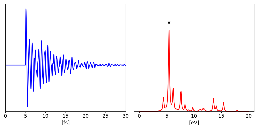
Notice that we introduced a scissor operator in such a way to have the main excitonic peak at 6.1 eV in agreement with experimental measurements. In this input we set only the first field that is the probe, and we use a DELTA function as field in such a way to probe all the spectra. Then we can analyze the spectra with ypp -u:

nonlinear                        # [R] Non-linear response analysis
Xorder= 1                        # Max order of the response/exc functions
% TimeRange
-1.000000 |-1.000000 |         fs    # Time-window where processing is done
%
ETStpsRt= 200                    # Total Energy steps
% EnRngeRt
  0.00000 | 20.00000 |         eV    # Energy range
%
DampMode= "LORENTZIAN"           # Damping type ( NONE | LORENTZIAN | GAUSSIAN )
DampFactor= 0.100000       eV    # Damping parameter
PumpPATH= "none"           # Path of the simulation with the Pump only

and get the dielectric response. Hereafter we plot the polarization along the y-direction and the corresponding dielectric constant:

Now we start from the previous input cp yambo.in_probe yambo.in_pump and
modify it in order perform a calculation with the Pump field only: yambo_nl -u p -V nl -F yambo.in_pump. These result will be our reference field in the final analysis:

nloptics                         # [R] Non-linear spectroscopy
% NLBands
 3 |  6 |                           # [NL] Bands range 
%
NLverbosity= "high"              # [NL] Verbosity level (low | high)
NLstep= 5.00000           as    # [NL] Time step length
NLtime= 150.000000           fs    # [NL] Simulation Time
NLintegrator= "CRANKNIC"         # [NL] Integrator ("EULEREXP/RK2/RK4/RK2EXP/HEUN/INVINT/CRANKNIC")
NLCorrelation= "SEX"             # [NL] Correlation ("IPA/HARTREE/TDDFT/LRC/LRW/JGM/SEX")
NLLrcAlpha= 0.000000             # [NL] Long Range Correction
NLDamping= 0.000000        eV    # [NL] Damping (or dephasing)
#EvalCurrent                   # [NL] Evaluate the current
HARRLvcs=  913             RL    # [HA] Hartree     RL components
EXXRLvcs=  913             RL    # [XX] Exchange    RL components
% GfnQP_E
 3.594325 | 1.000000 | 1.000000 |        # [EXTQP G] E parameters  (c/v) eV|adim|adim
%
% Field1_Freq
 0.100000 | 0.100000 |         eV    # [RT Field1] Frequency
%
Field1_Int=  1000.00       kWLm2 # [RT Field1] Intensity
Field1_Width= 0.000000     fs    # [RT Field1] Width
Field1_kind= "DELTA"             # [RT Field1] Kind(SIN|RES|ANTIRES|GAUSS|DELTA|QSSIN)
Field1_pol= "linear"             # [RT Field1] Pol(linear|circular)
% Field1_Dir
 0.000000 | 1.000000 | 0.000000 |        # [RT Field1] Versor
%
% Field1_Dir_circ
 0.000000 | 0.000000 | 0.000000 |        # [RT Field1] Versor_circ
%
Field1_Tstart= 165.00000    fs    # [RT Field1] Initial Time
% Field2_Freq
 6.1 | 6.1 |         eV    # [RT Field2] Frequency
%
Field2_Int= 1.E4      kWLm2 # [RT Field2] Intensity
Field2_Width= 10.000000     fs    # [RT Field2] Width
Field2_kind= "QSSIN"              # [RT Field2] Kind(SIN|RES|ANTIRES|GAUSS|DELTA|QSSIN)
Field2_pol= "linear"             # [RT Field2] Pol(linear|circular)
% Field2_Dir
 0.000000 | 1.000000 | 0.000000 |        # [RT Field2] Versor
%
% Field2_Dir_circ
 0.000000 | 0.000000 | 0.000000 |        # [RT Field2] Versor_circ
%
Field2_Tstart= 0.00000    fs    # [RT Field2] Initial Time

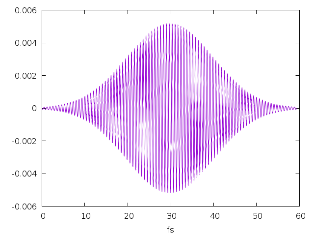
We set the starting time of the Probe (Field1) to 165 fs, a time larger then the simulation run in such a way to have only the Pump(Field2) field. As Pump field we use QSSIN that is an sine-Gaussian wave, with a frequency 6.1 eV centered at the energy of the first exciton, and a width of 10 fs: