Yambopy tutorial: band structures: Difference between revisions
No edit summary |
|||
| Line 7: | Line 7: | ||
==Tutorial 1. BN (semiconductor). Band structure== | ==Tutorial 1. BN (semiconductor). Band structure== | ||
The qepy classes are useful not only to execute Quantum Espresso but also to analyze the results. | The qepy classes are useful not only to execute Quantum Espresso but also to analyze the results. The full qepy library is imported by simply doing: | ||
from qepy import * | |||
'''Plot Band structure''' | '''Plot Band structure''' | ||
| Line 13: | Line 15: | ||
The class '''PwXML''' reads the data file generated by Quantum Espresso and post-process the data. The class is initiated doing: | The class '''PwXML''' reads the data file generated by Quantum Espresso and post-process the data. The class is initiated doing: | ||
xml = PwXML(prefix='bn', path='bands') | |||
The variable prefix corresponds to the same variable of the QE input. The folder location is indicated by variable path. | The variable prefix corresponds to the same variable of the QE input. The folder location is indicated by variable path. Previously to plot the bands, we define the k-points path using the function Path: | ||
npoints = 50 | |||
path_kpoints = Path([ [[0.0, 0.0, 0.0],'$\Gamma$'], | |||
[[0.5, 0.0, 0.0],'M'], | |||
[[1./3,1./3,0.0],'K'], | |||
[[0.0, 0.0, 0.0],'$\Gamma$']], [int(npoints*2),int(npoints),int(sqrt(5)*npoints)]) | |||
It is worth to note that the path should coincide with the selected path for the QE calculations. | |||
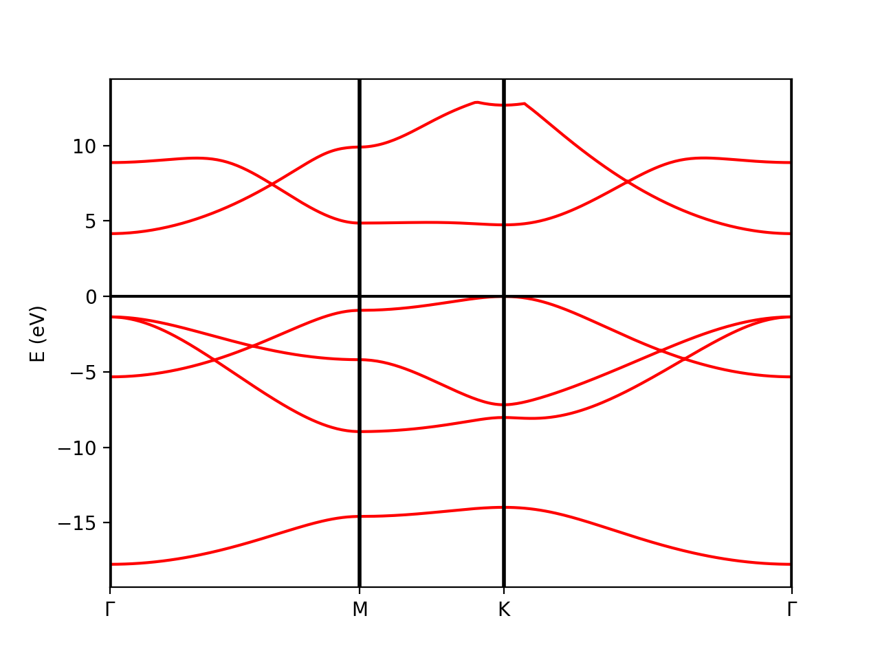
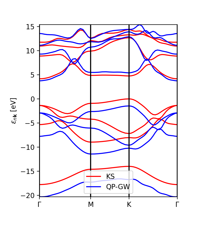
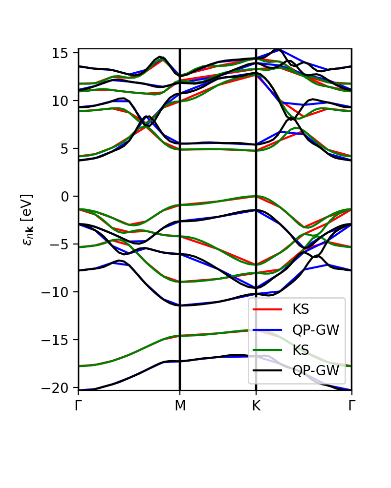
[[File:Bands BN 1.png| 400 px |Band structure of BN calculated at the level of DFT-LDA]] | [[File:Bands BN 1.png| 400 px |Band structure of BN calculated at the level of DFT-LDA]] | ||
Revision as of 14:31, 4 April 2022
The full tutorial, including the Quantum espresso and Yambo databases that we will read, can be downloaded and extracted from the yambo website:
$wget www.yambo-code.org/educational/tutorials/files/databases_qepy.tar
$tar -xvf databases_qepy.tar
$cd databases_qepy
Tutorial 1. BN (semiconductor). Band structure
The qepy classes are useful not only to execute Quantum Espresso but also to analyze the results. The full qepy library is imported by simply doing:
from qepy import *
Plot Band structure
The class PwXML reads the data file generated by Quantum Espresso and post-process the data. The class is initiated doing:
xml = PwXML(prefix='bn', path='bands')
The variable prefix corresponds to the same variable of the QE input. The folder location is indicated by variable path. Previously to plot the bands, we define the k-points path using the function Path:
npoints = 50
path_kpoints = Path([ [[0.0, 0.0, 0.0],'$\Gamma$'],
                      [[0.5, 0.0, 0.0],'M'],
                      [[1./3,1./3,0.0],'K'],
                      [[0.0, 0.0, 0.0],'$\Gamma$']], [int(npoints*2),int(npoints),int(sqrt(5)*npoints)])
It is worth to note that the path should coincide with the selected path for the QE calculations.
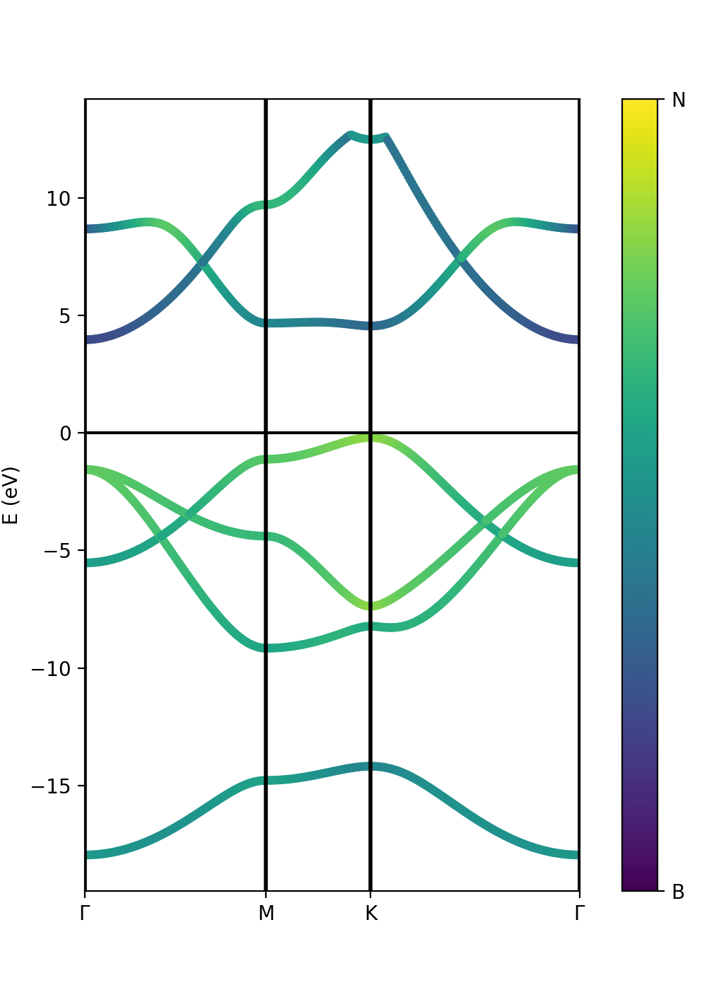
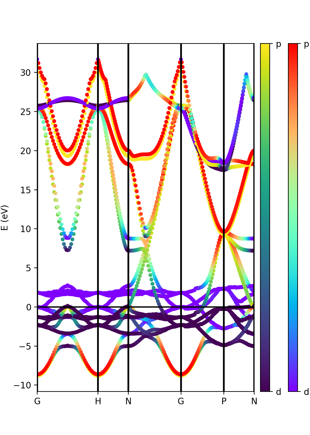
Plot atomic orbital projected Band structure
Tutorial 2
Tutorial 3
Links
- Back to ICTP 2022#Tutorials
