Pump and Probe: Difference between revisions
No edit summary |
No edit summary |
||
| Line 9: | Line 9: | ||
We start from the bulk hBN with an in place lattice constant a=4.72431525 a.u. and c/a=2.6. Standard DFT input for hBN | We start from the bulk hBN with an in place lattice constant a=4.72431525 a.u. and c/a=2.6. Standard DFT input for hBN | ||
for ABINIT or QuantumEspresso can be found here [[Tutorials]]. We used 200 bands in the Non-self consistent calculation. | for ABINIT or QuantumEspresso can be found here [[Tutorials]]. We used 200 bands in the Non-self consistent calculation. | ||
In our example we choose direction [0,1,0] for the pump and the probe. We generate the ypp.in to remove symmetries with the command <span style="color:blue">ypp -y</span> and we modify it as: | In our example we choose direction [0,1,0] for the pump and the probe. We generate the ypp.in to remove symmetries with the command <span style="color:blue">ypp -y</span> and we modify it as: | ||
| Line 27: | Line 26: | ||
#RmSpaceInv # Remove Spatial Inversion | #RmSpaceInv # Remove Spatial Inversion | ||
then we go in the | then we go in the FixSymm directory and run again the setup. | ||
then we generate the Pump&Probe input with the command <span style="color:blue">yambo_nl -u p -V rt</span>: | then we generate the Pump&Probe input with the command <span style="color:blue">yambo_nl -u p -V rt</span>: | ||
Revision as of 14:35, 10 January 2022
This tutorial works only with Yambo version > 5.0, that will be released soon.
In this tutorial we will show you how to setup two external fields in yambo_nl, to perform pump and probe simulation.
The input simulation parameters of these tutorial require large computational power,
we advice you to run them in parallel, or to use simplified parameters for example less bands, k-points and so on.
This tutorial supposes that you are already familiar with real-time simulation with Yambo,
if it is not the case please check these tutorials: Tutorials#Non_linear_response
We start from the bulk hBN with an in place lattice constant a=4.72431525 a.u. and c/a=2.6. Standard DFT input for hBN for ABINIT or QuantumEspresso can be found here Tutorials. We used 200 bands in the Non-self consistent calculation.
In our example we choose direction [0,1,0] for the pump and the probe. We generate the ypp.in to remove symmetries with the command ypp -y and we modify it as:
fixsyms                          # [R] Remove symmetries not consistent with an external perturbation
% Efield1
 0.000000 | 1.000000 | 0.000000 |        # First external Electric Field
%
% Efield2
 0.000000 | 1.000000 | 0.000000 |        # Additional external Electric Field
%
BField= 0.000000           T     # [MAG] Magnetic field modulus
Bpsi= 0.000000             deg   # [MAG] Magnetic field psi angle [degree]
Btheta= 0.000000           deg   # [MAG] Magnetic field theta angle [degree]
#RmAllSymm                     # Remove all symmetries
RmTimeRev                     # Remove Time Reversal
#RmSpaceInv                    # Remove Spatial Inversion
then we go in the FixSymm directory and run again the setup. then we generate the Pump&Probe input with the command yambo_nl -u p -V rt:
nloptics                         # [R] Non-linear spectroscopy
DIP_Threads=0                    # [OPENMP/X] Number of threads for dipoles
NL_Threads=0                     # [OPENMP/NL] Number of threads for nl-optics
% NLBands
   3 |  6 |                           # [NL] Bands range
%
NLverbosity= "high"              # [NL] Verbosity level (low | high)
NLstep= 0.010000           fs    # [NL] Time step length
NLtime= 75.0000         fs      # [NL] Simulation Time
NLintegrator= "INVINT"           # [NL] Integrator ("EULEREXP/RK2/RK4/RK2EXP/HEUN/INVINT/CRANKNIC")
NLCorrelation= "IPA"             # [NL] Correlation ("IPA/HARTREE/TDDFT/LRC/LRW/JGM/SEX")
NLLrcAlpha= 0.000000             # [NL] Long Range Correction
NLDamping= 0.100000        eV      # [NL] Damping (or dephasing)
RADLifeTime= 15.00000      fs      # [RT] Radiative life-time (if negative Yambo sets it equal to Phase_LifeTime in NL)
#UseDipoles                    # [NL] Use Covariant Dipoles (just for test purpose)
#FrSndOrd                      # [NL] Force second order in Covariant Dipoles
#EvalCurrent                   # [NL] Evaluate the current
HARRLvcs= 10417            RL    # [HA] Hartree     RL components
EXXRLvcs= 10417            RL    # [XX] Exchange    RL components
% ExtF_Dir
  1.000000 | 1.000000 | 0.000000 |        # [NL ExtF] Field Versor
%
% ExtF_Freq
  1.500000 | 1.500000 |         eV    # [NL ExtF] Field Frequency
%
ExtF_Int=  1000.00         kWLm2  # [NL ExtF] Field Intensity
ExtF_Width= 5.00000       fs    # [NL ExtF] Field Width
ExtF_kind= "QSSIN"               # [NL ExtF] Kind(SIN|SOFTSIN|RES|ANTIRES|GAUSS|DELTA|QSSIN)
ExtF_Tstart= 0.010000      fs    # [NL ExtF] Initial Time
% ExtF2_Dir
  0.000000 | 0.000000 | 1.000000 |        # [NL ExtF] Field Versor
%
% ExtF2_Freq
 0.100000 | 0.100000 |         eV    # [NL ExtF] Field Frequency
%
ExtF2_Int= 10.0000        kWLm2 # [NL ExtF] Field Intensity
ExtF2_Width= 0.000000      fs    # [NL ExtF] Field Width
ExtF2_kind= "DELTA"              # [NL ExtF] Kind(SIN|SOFTSIN|RES|ANTIRES|GAUSS|DELTA|QSSIN)
ExtF2_Tstart= 30.00000     fs    # [NL ExtF] Initial Time
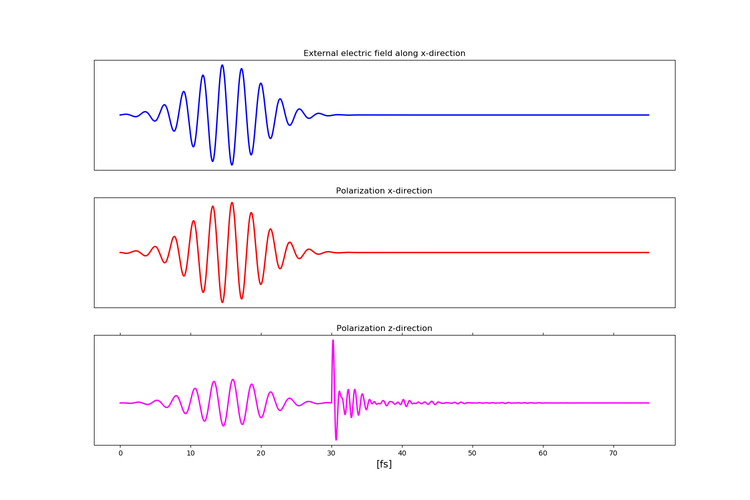
In this simulation we set a dephasing of 0.1 eV and a radiative life-time of 15 fs, The two external field are a sinus with frequency 1.5 eV convoluted with a Guassian of width 5 fs with and intensity of 1000 KW/cm-2, and then a delta function that starts at 30 fs with an intensity of 10 KW/cm-2. Below we plot the external electric field in the x direction and the polarization in x and z directions:
