Bethe-Salpeter on top of quasiparticle energies

In this module, you will learn how to include GW-corrected (QP) energies in the calculation of the absorption spectrum. The energy differences on the diagonal of the excitonic Hamiltonian are added before the solution of the Bethe-Salpeter eigenproblem, therefore only that step needs to be repeated if we change the QP corrections.

Prerequisites

Previous modules You must have completed

• the BSE kernel tutorial
• Optionally, the Bethe-Salpeter solver: diagonalization tutorial, in which a simple scissor operator is used for the QP corrections.

You will need:

• The SAVE databases for 3D hBN
• The ndb.BS_Q1_CPU_0 and ndb.em1s* databases for 3D hBN
• The ndb.QP database containing the GW-corrected band energies
• yambo executable

Reading the QP corrections from a previous GW calculation

In this previous calculation we have used a simple scissor operator to correct the Kohn-Sham DFT energies. In this part, we see how we can instead take the corrections from a previous Yambo GW calculation. We create and edit the input:

$yambo -F 03_3D_QP_BSE.in -y d -V qp -J 3D_BSE

We set all parameters as in the previous calculation, except for the part regarding the QP correction:

 KfnQPdb= "E < 3D_QP_BSE/ndb.QP"              # [EXTQP BSK BSS] Database
 KfnQP_N= 1                   # [EXTQP BSK BSS] Interpolation neighbours
 % KfnQP_E
  0.000000 | 1.000000 | 1.000000 |        # [EXTQP BSK BSS] E parameters  (c/v) eV|adim|adim
%

Instead of setting the values for the scissor, we give the path to a database (../GW_QP_database/ndb.QP), which contains the QP corrections. This has been created by running a GW calculation as in Step 3 of the GW tutorial. Run Yambo:

$ yambo -F 03_3D_QP_BSE.in -J "3D_QP_BSE,3D_BSE"

Note how we specified two directories, separated by a comma. This instructs Yambo to look for databases that may be already present from previous steps of the calculations in all the listed folders. If you completed the previous section of the tutorial, then you should have the 3D_BSE folder with ndb.dipoles_*, ndb.em1s* and ndb.BS_CPU* databases, which will not be recalculated by Yambo: the code will repeat only the diagonalization step, and print the resulting databases in the new folder 3D_QP_BSE. If you don't have the 3D_BSE folder, you have to repeat the entire BSE calculation, therefore you just need to give the option "-J 3D_QP_BSE".

This produces the following log in the standard output. Note Section 4 (regarding external QP corrections to the kernel):

<---> [04] External/Internal QP corrections
<---> E<../GW_QP_database/ndb.QP[ PPA@E  27.21138 = XG 5 = Xb 1-40 = Scb 1-40]
<---> [dE_from_DB-Nearest K] Exact matches       :  100.0000 [o/o]

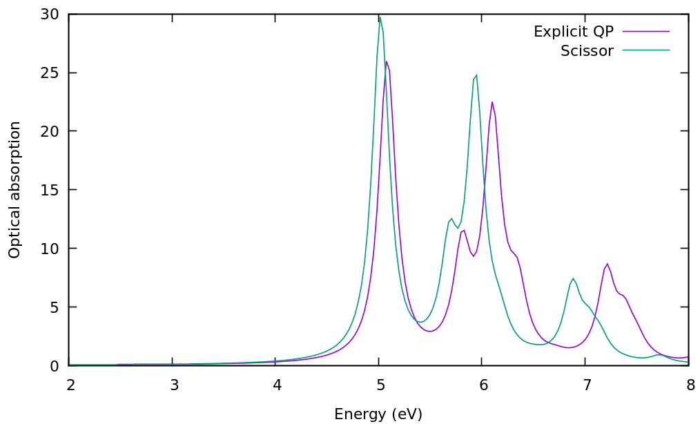
This tells you that the file was found, read correctly and that the k points found in the file matched the ones you are using for the current calculation (otherwise interpolation would be needed). It is crucial to check that the file has been read, since if not Yambo gives a warning but continues the calculation (with no QP corrections at all!). As in the calculation with the scissor shift the final results are the files with the spectral functions. Let's compare the results for the optical absorption spectrum with those obtained previously with a simple scissor:

$ gnuplot
...
plot 'o-3D_QP_BSE.eps_q1_diago_bse' u 1:2 w l t 'Explicit QP', 'o-3D_BSE.eps_q1_diago_bse' u 1:2 w l t 'Scissor' 

It is clear that this makes a difference in the peak positions, distribution and intensity. Note that besides a simple shift you can renormalise as well the bandwidth of the valence and conduction bands in KfnQP_E (respectively the third and second value). You can try as an exercise to set up a new calculation using e.g. 1.44 | 1.200000 | 0.900000 | for KfnQP_E.

Summary

From this tutorial you've learned:

• How to compute the optical spectrum including quasiparticle corrections (full GW+BSE calculation).

Links

• Previous module: Bethe-Salpeter solver: diagonalization
• Back to Calculating optical spectra including excitonic effects: a step-by-step guide tutorial
• Back to tutorials menu
• Back to technical modules menu