Generating the Yambo databases: Difference between revisions
mNo edit summary |
mNo edit summary |
||
| Line 1: | Line 1: | ||
== UNDER CONSTRUCTION (CH) == | == UNDER CONSTRUCTION (CH) == | ||
UNPACK IN SAME PLACE | |||
In this tutorial we will give a step-by-step demonstration how to generate the Yambo databases starting from a PWscf calculation. | In this tutorial we will give a step-by-step demonstration how to generate the Yambo databases starting from a PWscf calculation. | ||
== Prerequisites == | == Prerequisites == | ||
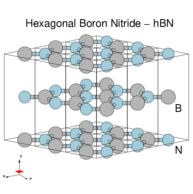
[[File:HBN-bulk-3x3-annotated.png|thumb|Atomic structure of bulk hBN]] | [[File:HBN-bulk-3x3-annotated.png|thumb|Atomic structure of bulk hBN]] | ||
== | '''Material properties''': | ||
== | * HCP lattice, ABAB stacking | ||
== | * Four atoms per cell, B and N (16 electrons, ) | ||
<code>p2y</code> ( | * Lattice constants: ''a'' = 4.716 [a.u.], ''c/a'' = 2.582 | ||
* Plane wave cutoff 40 Ry (1500 RL vectors in wavefunctions) | |||
'''You will need''': | |||
* PWSCF input files and pseudopotentials for hBN bulk (Download here) | |||
* <code>pw.x</code> executable, version 5.0 or later | |||
* <code>p2y</code> executable | |||
Unpack the TARFILE: | |||
$ tar -xcvf hBN-bulk.tar | |||
$ cd hBN/PWSCF | |||
$ ls | |||
hbn_bands.in hbn_nscf.in hbn_scf.in hbn_scf_b.in REFERENCES | |||
== DFT calculations == | |||
First run the SCF calculation in the usual manner, e.g. | |||
pw.x < hBN_scf.in > hBN_scf.out | |||
and then the non-SCF calculation to generate a set of Kohn-Sham eigenvalues and eigenvectors across a denser k-point mesh and for occupied and unoccupied states: | |||
pw.x < hBN_nscf.in > hBN_nscf.out | |||
Note the presence of the following flags in the input file: | |||
wf_collect=.true. | |||
force_symmorphic=.true. | |||
which are needed for the next step. Full explanations of these variables are given on the [http://www.quantum-espresso.org/wp-content/uploads/Doc/INPUT_PW.html quantum-ESPRESSO input variables page]. After these two runs, you should have a <code>hBN.save</code> directory: | |||
$ ls hBN.save | |||
data-file.xml | |||
== Conversion to Yambo format == | |||
PWscf output is converted to the Yambo format using the <code>p2y</code> (pwscf to yambo), found in the yambo <code>bin</code> directory. | |||
Enter the <code>hbn.save</code> directory and launch <code>p2y</code>: | |||
$ cd hBN.save | $ cd hBN.save | ||
$ p2y | $ p2y | ||
[output] | [output] | ||
The code reports some information about the system and generates a <code>SAVE</code> directory: | |||
$ ls | |||
$ ls | SAVE HB,in etc | ||
SAVE | |||
$ ls SAVE | $ ls SAVE | ||
ns.db1 ns.wf ns.kb_pp_pwscf | ns.db1 ns.wf ns.kb_pp_pwscf | ||
ns.wf_fragments_1_1 ... | ns.wf_fragments_1_1 ... | ||
ns.kb_pp_pwscf_fragment_1 ... | ns.kb_pp_pwscf_fragment_1 ... | ||
Finally, let's move the SAVE directory into a new clean folder: | |||
mv SAVE ../YAMBO/ | |||
== Advanced users == | |||
<code>p2y<code> accepts several command line options: | |||
$ p2y -H | |||
dfadsfas | |||
---- | ---- | ||
Next tutorial: [Introduction to yambo: input, output and command line interface] | Next tutorial: [[Introduction to yambo: input, output and command line interface]] | ||
Revision as of 16:28, 14 March 2017
UNDER CONSTRUCTION (CH)
UNPACK IN SAME PLACE
In this tutorial we will give a step-by-step demonstration how to generate the Yambo databases starting from a PWscf calculation.
Prerequisites
Material properties:
- HCP lattice, ABAB stacking
- Four atoms per cell, B and N (16 electrons, )
- Lattice constants: a = 4.716 [a.u.], c/a = 2.582
- Plane wave cutoff 40 Ry (1500 RL vectors in wavefunctions)
You will need:
- PWSCF input files and pseudopotentials for hBN bulk (Download here)
pw.xexecutable, version 5.0 or laterp2yexecutable
Unpack the TARFILE:
$ tar -xcvf hBN-bulk.tar
$ cd hBN/PWSCF
$ ls
hbn_bands.in	hbn_nscf.in hbn_scf.in	hbn_scf_b.in REFERENCES
DFT calculations
First run the SCF calculation in the usual manner, e.g.
pw.x < hBN_scf.in > hBN_scf.out
and then the non-SCF calculation to generate a set of Kohn-Sham eigenvalues and eigenvectors across a denser k-point mesh and for occupied and unoccupied states:
pw.x < hBN_nscf.in > hBN_nscf.out
Note the presence of the following flags in the input file:
wf_collect=.true.
force_symmorphic=.true.
which are needed for the next step. Full explanations of these variables are given on the quantum-ESPRESSO input variables page. After these two runs, you should have a hBN.save directory:
$ ls hBN.save
data-file.xml
Conversion to Yambo format
PWscf output is converted to the Yambo format using the p2y (pwscf to yambo), found in the yambo bin directory.
Enter the hbn.save directory and launch p2y:
$ cd hBN.save
$ p2y
[output]
The code reports some information about the system and generates a SAVE directory:
$ ls
SAVE HB,in etc
$ ls SAVE
ns.db1 ns.wf ns.kb_pp_pwscf
ns.wf_fragments_1_1 ...
ns.kb_pp_pwscf_fragment_1 ...
Finally, let's move the SAVE directory into a new clean folder:
mv SAVE ../YAMBO/
Advanced users
p2y accepts several command line options:
$ p2y -H
dfadsfas
Next tutorial: Introduction to yambo: input, output and command line interface
