Next steps: RPA calculations (standalone): Difference between revisions
| (17 intermediate revisions by 3 users not shown) | |||
| Line 1: | Line 1: | ||
==Optical absorption in hBN: independent particle approximation == | ==Optical absorption in hBN: independent particle approximation == | ||
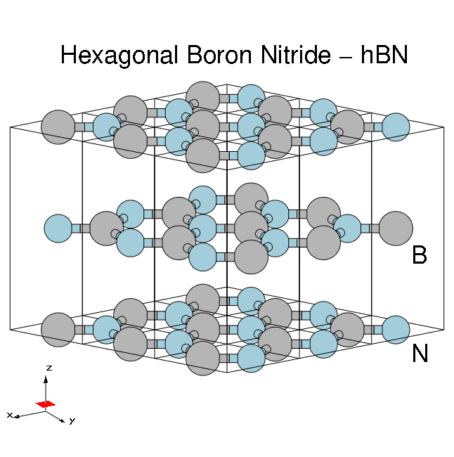
[[File:HBN-bulk-3x3-annotated.png|x200px|Atomic structure of bulk hBN]] | |||
=== Background === | === Background === | ||
The dielectric function in the long-wavelength limit, at the independent particle level (RPA without local fields), is essentially given by the following: | The dielectric function in the long-wavelength limit, at the independent particle level (RPA without local fields), is essentially given by the following: | ||
[ | |||
In practice, Yambo does not use this expression directly but solves the Dyson equation for the susceptibility | <math>\epsilon_{\alpha, \alpha}(\omega)=1+\frac{16 \pi}{\Omega} \sum_{c, v} \sum_{\mathbf{k}} \frac{1}{E_{c \mathbf{k}}-E_{v \mathbf{k}}} \frac{\left|\left\langle v \mathbf{k}\left|\mathbf{p}_{\alpha}+\mathrm i\left[V^{\mathrm{NL}}, \mathbf{r}_{\alpha}\right]\right| c \mathbf{k}\right\rangle\right|^{2}}{\left(E_{c \mathbf{k}}-E_{v \mathbf{k}}\right)^{2}-(\omega+\mathrm i \gamma)^{2}}</math> | ||
In practice, Yambo does not use this expression directly but solves the Dyson equation for the susceptibility <math>\chi</math>, which is described in the [[Local fields]] module. | |||
=== Choosing input parameters === | === Choosing input parameters === | ||
Enter the folder for bulk hBN that contains the ''SAVE'' directory, run the initialization and generate the input file. | Enter the folder for bulk hBN that contains the ''SAVE'' directory, run the initialization and generate the input file. | ||
You can type <code>yambo -h</code> and see the available options for different run-levels. For an RPA optical spectrum calculation the correct option is <code>yambo -optics c</code> (or <code>yambo -o c</code>). Let's add some command line options: | |||
$ cd YAMBO_TUTORIALS/hBN/YAMBO | $ cd YAMBO_TUTORIALS/hBN/YAMBO | ||
| Line 16: | Line 20: | ||
===Optics runlevel=== | ===Optics runlevel=== | ||
For optical properties we are interested just in the long-wavelength limit | For optical properties we are interested just in the long-wavelength limit <math>\mathbf q = 0</math>. This always corresponds to the ''first'' <math>\mathbf q</math>-point in the set of possible <math>\mathbf q =\mathbf k - \mathbf k'</math>-points. | ||
Change the following variables in the input file to: | Change the following variables in the input file to: | ||
% [[Variables#QpntsRX|QpntsRXd]] | % [[Variables#QpntsRX|QpntsRXd]] | ||
| Line 22: | Line 26: | ||
% | % | ||
[[Variables#ETStpsX|ETStpsXd]]= '''1001''' # [Xd] Total Energy steps | [[Variables#ETStpsX|ETStpsXd]]= '''1001''' # [Xd] Total Energy steps | ||
in order to select just the first | in order to select just the first <math>\mathbf q</math>. The last variable ensures we generate a smooth spectrum. | ||
Save the input file and launch the code, keeping the command line options as before (i.e., just remove the lower case options): | Save the input file and launch the code, keeping the command line options as before (i.e., just remove the lower case options): | ||
$ yambo -F yambo.in_IP -J Full | $ yambo -F yambo.in_IP -J Full | ||
| Line 29: | Line 33: | ||
<---> [LA] SERIAL linear algebra | <---> [LA] SERIAL linear algebra | ||
<---> [DIP] Checking dipoles header | <---> [DIP] Checking dipoles header | ||
<--- | <---> [X-CG] R(p) Tot o/o(of R): 5499 52992 100 | ||
<02s> Xo@q[1] |########################################| [100%] --(E) --(X) | |||
<02s> [06] Timing Overview | |||
<02s> [07] Memory Overview | |||
<02s> [08] Game Over & Game summary | |||
< | |||
< | |||
$ ls | $ ls | ||
| Line 43: | Line 43: | ||
o-Full.eel_q1_ip o-Full.eps_q1_ip r-Full_optics_chi | o-Full.eel_q1_ip o-Full.eps_q1_ip r-Full_optics_chi | ||
Let's take a moment to understand what Yambo has done inside the Optics runlevel: | Let's take a moment to understand what Yambo has done inside the Optics runlevel: | ||
# Compute the | # Compute the <math>[\mathbf r, V^\mathrm{NL}]</math> term | ||
# Read the wavefunctions from disc [WF] | # Read the wavefunctions from disc [WF] | ||
# Compute the ''dipoles'', i.e. matrix elements of | # Compute the ''dipoles'', i.e. matrix elements of <math>\mathbf p</math> | ||
# Write the dipoles to disk as ''Full/ndb.dip*'' databases. This you can see in the report file: | # Write the dipoles to disk as ''Full/ndb.dip*'' databases. This you can see in the report file: | ||
$ grep -A20 "WR" r- | $ grep -A20 "WR" r-Full_optics_* | ||
[WR./Full//ndb. | [WR./Full//ndb.dipoles]--------------------------------------------------------- | ||
Brillouin Zone Q/K grids (IBZ/BZ) : 14 72 14 72 | |||
RL vectors : 1491 [WF] | |||
Fragmentation : yes | |||
Electronic Temperature : 0.000000 [K] | |||
Bosonic Temperature : 0.000000 [K] | |||
DIP band range : 1 100 | |||
DIP band range limits : 8 9 | |||
DIP e/h energy range : -1.000000 -1.000000 [eV] | |||
RL vectors in the sum : 1491 | |||
[r,Vnl] included : yes | |||
... | |||
<ol start="5"> | <ol start="5"> | ||
<li>Finally, Yambo computes the non-interacting susceptibility | <li>Finally, Yambo computes the non-interacting susceptibility <math>\chi</math> for this <math>\mathbf q</math>, and writes the dielectric function inside the ''o-Full.eps_q1_ip'' file for plotting</li> | ||
</ol> | </ol> | ||
| Line 64: | Line 68: | ||
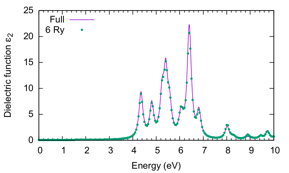
Before plotting the output, let's change a few more variables. The previous calculation used ''all'' the G-vectors in expanding the wavefunctions, up to 1491 (~1016 components). This corresponds roughly to the cut off energy of 40Ry we used in the DFT calculation. Generally, however, we can use a smaller value. We use the verbosity to switch on this variable, and a new ''-J'' flag to avoid reading the previous database: | Before plotting the output, let's change a few more variables. The previous calculation used ''all'' the G-vectors in expanding the wavefunctions, up to 1491 (~1016 components). This corresponds roughly to the cut off energy of 40Ry we used in the DFT calculation. Generally, however, we can use a smaller value. We use the verbosity to switch on this variable, and a new ''-J'' flag to avoid reading the previous database: | ||
$ yambo -F yambo.in_IP ''' | $ yambo -F yambo.in_IP '''-V RL''' -o c | ||
Change the '''value''' of <code>[[Variables#FFTGvecs|FFTGvecs]]</code> and also its '''unit''' from <code>RL</code> (number of G-vectors) to <code>Ry</code> (energy in Rydberg): | Change the '''value''' of <code>[[Variables#FFTGvecs|FFTGvecs]]</code> and also its '''unit''' from <code>RL</code> (number of G-vectors) to <code>Ry</code> (energy in Rydberg): | ||
[[Variables#FFTGvecs|FFTGvecs]]= '''6''' '''Ry''' # [FFT] Plane-waves | [[Variables#FFTGvecs|FFTGvecs]]= '''6''' '''Ry''' # [FFT] Plane-waves | ||
| Line 75: | Line 79: | ||
[[File:CH-hBN-6Ry.png|none|500px|Yambo tutorial image]] | [[File:CH-hBN-6Ry.png|none|500px|Yambo tutorial image]] | ||
There is very little difference between the two spectra. This highlights an important point in calculating excited state properties: generally, fewer G-vectors are needed than what are needed in DFT calculations. Regarding the spectrum itself, the first peak occurs at about 4.4eV. This is consistent with the minimum direct gap reported by Yambo: 4.28eV. The comparison with experiment (not shown) is very poor however. | |||
If you | If you made some mistake and cannot reproduce this figure, you should check the value of <code>[[Variables#FFTGvecs|FFTGvecs]]</code> in the input file, delete the ''6Ry'' folder, and try again - taking care to plot the right file! (e.g. ''o-6Ry.eps_q1_ip_01''. The "_01" suffix means that while writing the output Yambo found another existing file with the name "o-6Ry.eps_q1_ip"). | ||
===q-direction=== | ===q-direction=== | ||
Now let's select a different component of the dielectric tensor: | Now let's select a different component of the dielectric tensor: | ||
$ yambo -F yambo.in_IP | $ yambo -F yambo.in_IP -V RL -o c | ||
... | ... | ||
% [[Variables#LongDrXd|LongDrXd]] | % [[Variables#LongDrXd|LongDrXd]] | ||
| Line 96: | Line 100: | ||
===Non-local commutator=== | ===Non-local commutator=== | ||
Last, we show the effect of switching off the non-local commutator term ( | Last, we show the effect of switching off the non-local commutator term (the term with <math> V^\mathrm{NL} </math> in the equation at the start of this tutorial) due to the pseudopotential. As there is no option to do this inside yambo, you need to hide the database file. Change back to the ''q || (1 0 0)'' direction, and launch yambo with a different <code>-J</code> option: | ||
$ mv SAVE/ns.kb_pp_pwscf SAVE/ns.kb_pp_pwscf_'''OFF''' | $ mv SAVE/ns.kb_pp_pwscf SAVE/ns.kb_pp_pwscf_'''OFF''' | ||
$ yambo -F yambo.in_IP -J '''6Ry_NoVnl''' -o c '' | $ yambo -F yambo.in_IP -J '''6Ry_NoVnl''' -o c | ||
Change | |||
%LonDrXd | |||
back to | |||
'''1.000000''' | 0.000000 | '''0.000000''' | | |||
and run | |||
$ yambo -F yambo.in_IP -J 6Ry_NoVnl | $ yambo -F yambo.in_IP -J 6Ry_NoVnl | ||
Note the warning in the output: | Note the warning in the output: | ||
<---> [WARNING] | <---> [WARNING] [r,Vnl^pseudo] not included in position and velocity dipoles | ||
which also appears in the report file | which also appears in the report file <code>r-6Ry_NoVnl_optics_dipoles_chi</code> as <code>[r,Vnl] included :no</code>. The difference is tiny: | ||
[[File:CH-hBN-Vnl.png|none|500px|Yambo tutorial image]] | [[File:CH-hBN-Vnl.png|none|500px|Yambo tutorial image]] | ||
However, when your system is larger, with more projectors in the pseudopotential or more k-points (see the BSE tutorial), the inclusion of | However, when your system is larger, with more projectors in the pseudopotential or more k-points (see the BSE tutorial), the inclusion of <math>V^\mathrm{NL}</math> can make a huge difference in the computational load, so it is always worth checking to see if the terms are important in your system. | ||
==Optical absorption in 2D BN: local field effects == | ==Optical absorption in 2D BN: local field effects == | ||
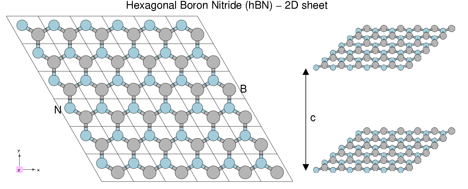
[[File:HBN2.png|x200px|Atomic structure of 2D hBN]] | |||
=== Background === | === Background === | ||
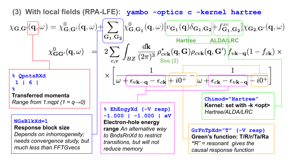
[[File:Yambo- | [[File:Yambo-Cheatsheet-5.0_P7.png|thumb|Cheatsheet on LFE|150px]] | ||
The macroscopic dielectric function is obtained by including the so-called local field effects (LFE) in the calculation of the response function. Within the time-dependent DFT formalism this is achieved by solving the Dyson equation for the susceptibility | The macroscopic dielectric function is obtained by including the so-called local field effects (LFE) in the calculation of the response function. Within the time-dependent DFT formalism this is achieved by solving the Dyson equation for the susceptibility <math>\chi</math>. In reciprocal space this is given by: | ||
[ | |||
The microscopic dielectric function is related to | <math>\chi_{\mathbf{G}, \mathbf{G}^{\prime}}(\mathbf{q}, \omega) = \chi_{\mathbf{G}, \mathbf{G}^{\prime}}^{0}(\mathbf{q}, \omega)+\sum_{\mathbf{G}_{1}, \mathbf{G}_{2}} \chi_{\mathbf{G}, \mathbf{G}_{1}}^{0}(\mathbf{q}, \omega)\left[v_{\mathbf{G}_{1}}(\mathbf{q}) \delta_{\mathbf{G}_{1}, \mathbf{G}_{2}}+f_{\mathbf{G}_{1}, \mathbf{G}_{2}}^{x c}\right] \chi_{\mathbf{G}_{2}, \mathbf{G}^{\prime}}(\mathbf{q}, \omega)</math> | ||
The microscopic dielectric function is related to <math>\chi</math> by: | |||
<math>\epsilon_{\mathbf{G}, \mathbf{G}^{\prime}}^{-1}(\mathbf{q}, \omega)=\delta_{\mathbf{G}, \mathbf{G}^{\prime}}+v_{\mathbf{G}}(\mathbf{q}) \chi_{\mathbf{G}, \mathbf{G}^{\prime}}(\mathbf{q}, \omega)</math> | |||
and the macroscopic dielectric function is obtained by taking the (0,0) component of the inverse microscopic one: | and the macroscopic dielectric function is obtained by taking the (0,0) component of the inverse microscopic one: | ||
<math>\epsilon_{M}(\omega)=\lim _{\mathrm{q} \rightarrow 0} \frac{1}{\epsilon_{\mathrm{G}=0, \mathrm{G}^{\prime}=0}^{-1}(\mathbf{q}, \omega)}</math> | |||
Experimental observables like the optical absorption and the electron energy loss can be obtained from the macroscopic dielectric function: | Experimental observables like the optical absorption and the electron energy loss can be obtained from the macroscopic dielectric function: | ||
In the following we will neglect the | <math>\operatorname{Abs}(\omega)=\operatorname{Im} \epsilon_{M}(\omega) \quad \operatorname{EELS}(\omega)=-\operatorname{Im} \frac{1}{\epsilon_{M}(\omega)}</math> | ||
In the following we will neglect the <math>f^{xc}</math> term: we perform the calculation at the RPA level and consider just the Hartree term (from <math>v_G</math>) in the kernel. If we also neglect the Hartree term, we arrive back at the independent particle approximation, since there is no kernel and <math>\chi = \chi_0</math>. | |||
=== Choosing input parameters === | === Choosing input parameters === | ||
Enter the folder for 2D hBN that contains the SAVE directory, and generate the input file. | Enter the folder for 2D hBN that contains the SAVE directory, and generate the input file. To include local the local fields variables in the input file the correct option is <code>yambo -o c -k hartree</code> (once again you can check it with <code>yambo -h</code>). Let's start by running the calculation for light polarization ''q'' in the plane of the BN sheet: | ||
$ cd YAMBO_TUTORIALS/hBN-2D/YAMBO | $ cd YAMBO_TUTORIALS/hBN-2D/YAMBO | ||
$ yambo ''(Initialization)'' | $ yambo ''(Initialization)'' | ||
$ yambo -F yambo.in_RPA -V RL | $ yambo -F yambo.in_RPA -V RL -o c -k hartree | ||
We thus use a new input file ''yambo.in_RPA'', switch on the <code>FFTGvecs</code> variable, and label all outputs/databases with a ''q100'' tag. Make sure to set/modify all of the following variables to: | We thus use a new input file ''yambo.in_RPA'', switch on the <code>FFTGvecs</code> variable, and label all outputs/databases with a ''q100'' tag. Make sure to set/modify all of the following variables to: | ||
[[Variables#FFTGvecs|FFTGvecs]]= '''6 Ry''' # [FFT] Plane-waves | [[Variables#FFTGvecs|FFTGvecs]]= '''6 Ry''' # [FFT] Plane-waves | ||
| Line 132: | Line 158: | ||
[[Variables#NGsBlkXd|NGsBlkXd]]= ''' 3 Ry''' # [Xd] Response block size | [[Variables#NGsBlkXd|NGsBlkXd]]= ''' 3 Ry''' # [Xd] Response block size | ||
% [[Variables#QpntsRXd|QpntsRXd]] | % [[Variables#QpntsRXd|QpntsRXd]] | ||
1 | 1 | # [Xd] Transferred momenta | 1 | '''1''' | # [Xd] Transferred momenta | ||
% | % | ||
% [[Variables#EnRngeXd|EnRngeXd]] | % [[Variables#EnRngeXd|EnRngeXd]] | ||
0.00000 | 20.00000 | eV # [Xd] Energy range | 0.00000 | '''20.00000''' | eV # [Xd] Energy range | ||
% | % | ||
% [[Variables#DmRngeXd|DmRngeXd]] | % [[Variables#DmRngeXd|DmRngeXd]] | ||
0.200000 | 0.200000 | eV # [Xd] Damping range | '''0.200000''' | '''0.200000''' | eV # [Xd] Damping range | ||
% | % | ||
[[Variables#ETStpsXd|ETStpsXd]]= 2001 # [Xd] Total Energy steps | [[Variables#ETStpsXd|ETStpsXd]]= 2001 # [Xd] Total Energy steps | ||
| Line 144: | Line 170: | ||
1.000000 | 0.000000 | 0.000000 | # [Xd] [cc] Electric Field | 1.000000 | 0.000000 | 0.000000 | # [Xd] [cc] Electric Field | ||
% | % | ||
In this input file | In this input file: | ||
* We evaluate the q | * We evaluate the <math>\mathbf q \rightarrow 0</math> response function choosing the direction for the limit parallel in the plane of the hBN sheet; | ||
* | * We set a wider energy range than before, and a larger broadening; | ||
* | * We select the Hartree kernel, and expanded G-vectors in the screening up to 3 Ry (about 85 G-vectors); | ||
===LFEs in periodic direction=== | ===LFEs in periodic direction=== | ||
Now let's run the code with this new input file (CECAM in serial: about 2mins; parallel 4 tasks: 50s) | Now let's run the code with this new input file (CECAM in serial: about 2mins; parallel 4 tasks: 50s) | ||
$ yambo -F yambo.in_RPA -J q100 | $ yambo -F yambo.in_RPA -J q100 | ||
and let's compare the absorption with and without the local fields included. By inspecting the ''o-q100.eps_q1_inv_rpa_dyson'' file we find | and let's compare the absorption with and without the local fields included. By inspecting the ''o-q100.eps_q1_inv_rpa_dyson'' file we find that this information is given in the 2<math>^\mathrm{nd}</math> and 4<math>^\mathrm{th}</math> columns, respectively: | ||
that this information is given in the | $ head -n 40 o-q100.eps_q1_inv_rpa_dyson | ||
$ head - | |||
# Absorption @ Q(1) [q->0 direction] : 1.0000000 0.0000000 0.0000000 | # Absorption @ Q(1) [q->0 direction] : 1.0000000 0.0000000 0.0000000 | ||
# E/ev[1] EPS-Im[2] EPS-Re[3] EPSo-Im[4] EPSo-Re[5] | # E/ev[1] EPS-Im[2] EPS-Re[3] EPSo-Im[4] EPSo-Re[5] | ||
Plot the result: | Plot the result: | ||
$ gnuplot | $ gnuplot | ||
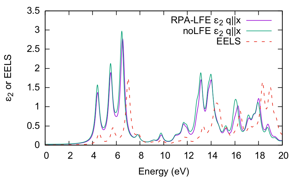
gnuplot> plot "o-q100.eps_q1_inv_rpa_dyson" u 1:2 w l t "RPA- | $ gnuplot> plot "o-q100.eps_q1_inv_rpa_dyson" u 1:2 w l t "RPA-LFE","o-q100.eps_q1_inv_rpa_dyson" u 1:4 w l t "noLFE", "o-q100.eel_q1_inv_rpa_dyson" u 1:4 w l ls 7 dt 2 t "EELS" | ||
[[File:CH-LFE4.png|none|600px|Yambo tutorial image]] | [[File:CH-LFE4.png|none|600px|Yambo tutorial image]] | ||
There is little influence of local fields in this case. This is generally the case for semiconductors or materials with a smoothly varying electronic density. We have also shown the EELS spectrum (''o-q100.eel_q1_inv_rpa_dyson'') for comparison. | |||
===LFEs in non-periodic direction=== | ===LFEs in non-periodic direction=== | ||
| Line 185: | Line 210: | ||
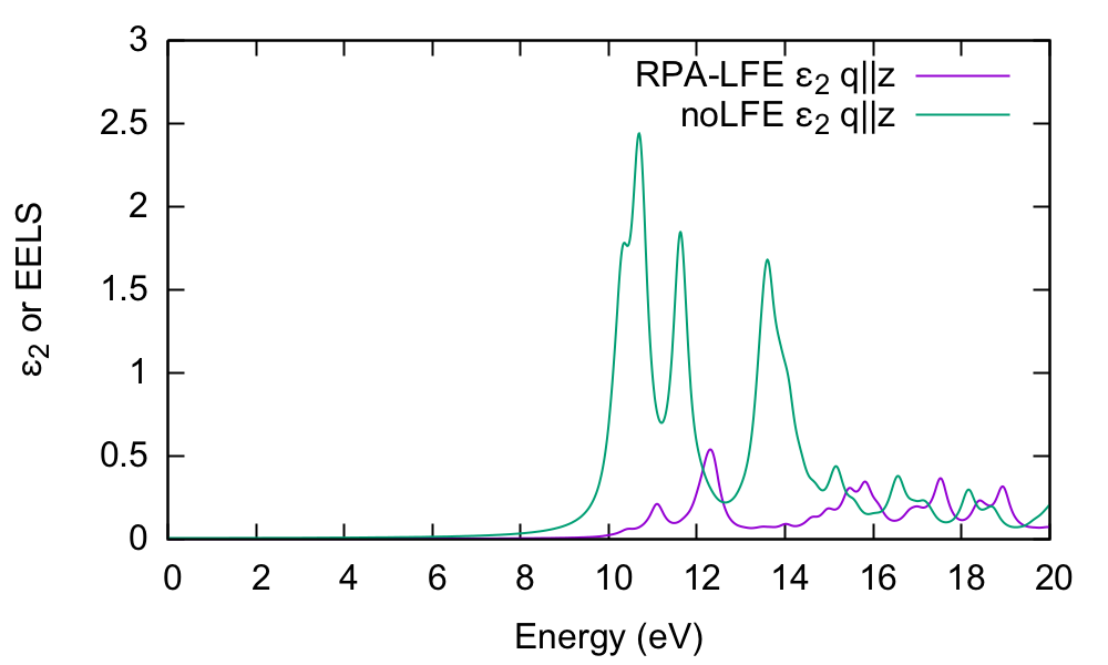
In order to understand this further, we plot the electron energy loss spectrum for this component and compare with the absorption: | In order to understand this further, we plot the electron energy loss spectrum for this component and compare with the absorption: | ||
$ gnuplot | $ gnuplot | ||
gnuplot > plot "o-q001.eps_q1_inv_rpa_dyson" w l,"o-q001.eel_q1_inv_rpa_dyson" w l | $ gnuplot > plot "o-q001.eps_q1_inv_rpa_dyson" w l,"o-q001.eel_q1_inv_rpa_dyson" w l | ||
[[File:CH-LFE5.png|none|600px|Yambo tutorial image]] | [[File:CH-LFE5.png|none|600px|Yambo tutorial image]] | ||
The conclusion is that the absorption and EELS coincide for isolated systems. | The conclusion is that the absorption and EELS coincide for isolated systems. | ||
| Line 191: | Line 216: | ||
See e.g.<ref>TDDFT from molecules to solids: The role of long‐range interactions, F. Sottile et al, International journal of quantum chemistry 102 (5), 684-701 (2005)</ref> | See e.g.<ref>TDDFT from molecules to solids: The role of long‐range interactions, F. Sottile et al, International journal of quantum chemistry 102 (5), 684-701 (2005)</ref> | ||
==Links== | |||
* Back to [[ICTP 2022#Tutorials]] | |||
* Back to [[CECAM VIRTUAL 2021#Tutorials]] | |||
<!-- | |||
<br> | <br> | ||
{| style="width:100%" border="1" | {| style="width:100%" border="1" | ||
|style="width:25%; text-align:left"|Prev: CECAM School Home | |style="width:25%; text-align:left"|Prev: CECAM School Home -> [[First_steps:_walk_through_from_DFT(standalone)|First steps]] | ||
|style="width:40%; text-align:center"|Now: CECAM School Home | |style="width:40%; text-align:center"|Now: CECAM School Home -> [[Next steps: RPA calculations (standalone)|Next steps]] | ||
|style="width:35%; text-align:right"|Back to: [[CECAM_VIRTUAL_2021#Tutorials|CECAM School Home]] | |style="width:35%; text-align:right"|Back to: [[CECAM_VIRTUAL_2021#Tutorials|CECAM School Home]] | ||
|- | |- | ||
|} | |} | ||
--> | |||
Latest revision as of 14:33, 20 May 2025
Optical absorption in hBN: independent particle approximation
Background
The dielectric function in the long-wavelength limit, at the independent particle level (RPA without local fields), is essentially given by the following:
[math]\displaystyle{ \epsilon_{\alpha, \alpha}(\omega)=1+\frac{16 \pi}{\Omega} \sum_{c, v} \sum_{\mathbf{k}} \frac{1}{E_{c \mathbf{k}}-E_{v \mathbf{k}}} \frac{\left|\left\langle v \mathbf{k}\left|\mathbf{p}_{\alpha}+\mathrm i\left[V^{\mathrm{NL}}, \mathbf{r}_{\alpha}\right]\right| c \mathbf{k}\right\rangle\right|^{2}}{\left(E_{c \mathbf{k}}-E_{v \mathbf{k}}\right)^{2}-(\omega+\mathrm i \gamma)^{2}} }[/math]
In practice, Yambo does not use this expression directly but solves the Dyson equation for the susceptibility [math]\displaystyle{ \chi }[/math], which is described in the Local fields module.
Choosing input parameters
Enter the folder for bulk hBN that contains the SAVE directory, run the initialization and generate the input file.
You can type yambo -h and see the available options for different run-levels. For an RPA optical spectrum calculation the correct option is yambo -optics c (or yambo -o c). Let's add some command line options:
$ cd YAMBO_TUTORIALS/hBN/YAMBO
$ yambo               (initialization)
$ yambo -F yambo.in_IP -o c
This corresponds to optical properties in G-space at the independent particle level: in the input file this is indicated by (Chimod= "IP").
Optics runlevel
For optical properties we are interested just in the long-wavelength limit [math]\displaystyle{ \mathbf q = 0 }[/math]. This always corresponds to the first [math]\displaystyle{ \mathbf q }[/math]-point in the set of possible [math]\displaystyle{ \mathbf q =\mathbf k - \mathbf k' }[/math]-points. Change the following variables in the input file to:
% QpntsRXd
 1 |  1 |                   # [Xd] Transferred momenta
%
ETStpsXd= 1001               # [Xd] Total Energy steps
in order to select just the first [math]\displaystyle{ \mathbf q }[/math]. The last variable ensures we generate a smooth spectrum. Save the input file and launch the code, keeping the command line options as before (i.e., just remove the lower case options):
$ yambo -F yambo.in_IP -J Full
...
<---> [05] Optics
<---> [LA] SERIAL linear algebra
<---> [DIP] Checking dipoles header
<---> [X-CG] R(p) Tot o/o(of R):    5499   52992     100
<02s> Xo@q[1] |########################################| [100%] --(E) --(X)
<02s> [06] Timing Overview
<02s> [07] Memory Overview
<02s> [08] Game Over & Game summary

$ ls
Full   SAVE  yambo.in_IP   r_setup
o-Full.eel_q1_ip  o-Full.eps_q1_ip  r-Full_optics_chi
Let's take a moment to understand what Yambo has done inside the Optics runlevel:
- Compute the [math]\displaystyle{ [\mathbf r, V^\mathrm{NL}] }[/math] term
- Read the wavefunctions from disc [WF]
- Compute the dipoles, i.e. matrix elements of [math]\displaystyle{ \mathbf p }[/math]
- Write the dipoles to disk as Full/ndb.dip* databases. This you can see in the report file:
$ grep -A20 "WR" r-Full_optics_*
[WR./Full//ndb.dipoles]---------------------------------------------------------
 Brillouin Zone Q/K grids (IBZ/BZ)                :   14   72   14   72
 RL vectors                                       :  1491 [WF]
 Fragmentation                                    : yes
 Electronic Temperature                           :  0.000000 [K]
 Bosonic    Temperature                           :  0.000000 [K]
 DIP band range                                   :    1  100
 DIP band range limits                            :   8   9
 DIP e/h energy range                             : -1.000000 -1.000000 [eV]
 RL vectors in the sum                            :  1491
 [r,Vnl] included                                 : yes
 ...
- Finally, Yambo computes the non-interacting susceptibility [math]\displaystyle{ \chi }[/math] for this [math]\displaystyle{ \mathbf q }[/math], and writes the dielectric function inside the o-Full.eps_q1_ip file for plotting
Energy cut off
Before plotting the output, let's change a few more variables. The previous calculation used all the G-vectors in expanding the wavefunctions, up to 1491 (~1016 components). This corresponds roughly to the cut off energy of 40Ry we used in the DFT calculation. Generally, however, we can use a smaller value. We use the verbosity to switch on this variable, and a new -J flag to avoid reading the previous database:
$ yambo -F yambo.in_IP -V RL -o c
Change the value of FFTGvecs and also its unit from RL (number of G-vectors) to Ry (energy in Rydberg):
FFTGvecs= 6 Ry # [FFT] Plane-waves
Save the input file and launch the code again:
$ yambo -F yambo.in_IP -J 6Ry
and then plot the o-Full.eps_q1_ip and o-6Ry.eps_q1_ip files:
$ gnuplot
gnuplot> plot "o-Full.eps_q1_ip" w l,"o-6Ry.eps_q1_ip" w p
There is very little difference between the two spectra. This highlights an important point in calculating excited state properties: generally, fewer G-vectors are needed than what are needed in DFT calculations. Regarding the spectrum itself, the first peak occurs at about 4.4eV. This is consistent with the minimum direct gap reported by Yambo: 4.28eV. The comparison with experiment (not shown) is very poor however.
If you made some mistake and cannot reproduce this figure, you should check the value of FFTGvecs in the input file, delete the 6Ry folder, and try again - taking care to plot the right file! (e.g. o-6Ry.eps_q1_ip_01. The "_01" suffix means that while writing the output Yambo found another existing file with the name "o-6Ry.eps_q1_ip").
q-direction
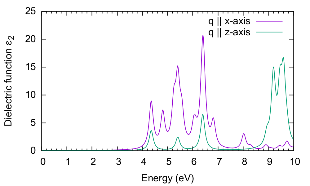
Now let's select a different component of the dielectric tensor:
$ yambo -F yambo.in_IP -V RL -o c
...
% LongDrXd
0.000000 | 0.000000 | 1.000000 |        # [Xd] [cc] Electric Field
%
...
$ yambo -F yambo.in_IP -J 6Ry
This time yambo reads from the 6Ry folder, so it does not need to compute the dipole matrix elements again, and the calculation is fast. Plotting gives:
$ gnuplot
gnuplot> plot "o-6Ry.eps_q1_ip" t "q || x-axis" w l,"o-6Ry.eps_q1_ip_01" t "q || c-axis" w l
The absorption is suppressed in the stacking direction. As the interplanar spacing is increased, we would eventually arrive at the absorption of the BN sheet (see Local fields tutorial).
Non-local commutator
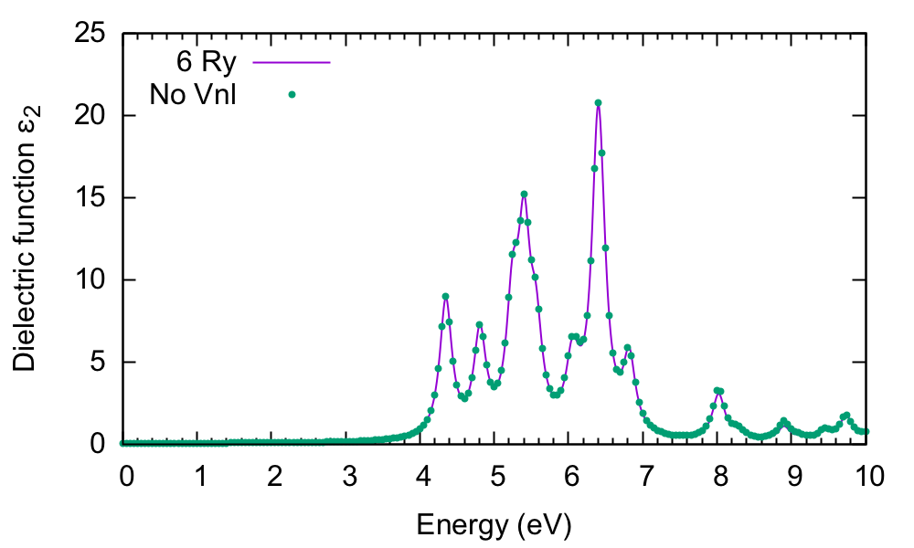
Last, we show the effect of switching off the non-local commutator term (the term with [math]\displaystyle{ V^\mathrm{NL} }[/math] in the equation at the start of this tutorial) due to the pseudopotential. As there is no option to do this inside yambo, you need to hide the database file. Change back to the q || (1 0 0) direction, and launch yambo with a different -J option:
$ mv SAVE/ns.kb_pp_pwscf SAVE/ns.kb_pp_pwscf_OFF
$ yambo -F yambo.in_IP -J 6Ry_NoVnl -o c
Change
%LonDrXd
back to
1.000000 | 0.000000 | 0.000000 |
and run
$ yambo -F yambo.in_IP -J 6Ry_NoVnl
Note the warning in the output:
<---> [WARNING] [r,Vnl^pseudo] not included in position and velocity dipoles
which also appears in the report file r-6Ry_NoVnl_optics_dipoles_chi as [r,Vnl] included :no. The difference is tiny:
However, when your system is larger, with more projectors in the pseudopotential or more k-points (see the BSE tutorial), the inclusion of [math]\displaystyle{ V^\mathrm{NL} }[/math] can make a huge difference in the computational load, so it is always worth checking to see if the terms are important in your system.
Optical absorption in 2D BN: local field effects
Background
The macroscopic dielectric function is obtained by including the so-called local field effects (LFE) in the calculation of the response function. Within the time-dependent DFT formalism this is achieved by solving the Dyson equation for the susceptibility [math]\displaystyle{ \chi }[/math]. In reciprocal space this is given by:
[math]\displaystyle{ \chi_{\mathbf{G}, \mathbf{G}^{\prime}}(\mathbf{q}, \omega) = \chi_{\mathbf{G}, \mathbf{G}^{\prime}}^{0}(\mathbf{q}, \omega)+\sum_{\mathbf{G}_{1}, \mathbf{G}_{2}} \chi_{\mathbf{G}, \mathbf{G}_{1}}^{0}(\mathbf{q}, \omega)\left[v_{\mathbf{G}_{1}}(\mathbf{q}) \delta_{\mathbf{G}_{1}, \mathbf{G}_{2}}+f_{\mathbf{G}_{1}, \mathbf{G}_{2}}^{x c}\right] \chi_{\mathbf{G}_{2}, \mathbf{G}^{\prime}}(\mathbf{q}, \omega) }[/math]
The microscopic dielectric function is related to [math]\displaystyle{ \chi }[/math] by:
[math]\displaystyle{ \epsilon_{\mathbf{G}, \mathbf{G}^{\prime}}^{-1}(\mathbf{q}, \omega)=\delta_{\mathbf{G}, \mathbf{G}^{\prime}}+v_{\mathbf{G}}(\mathbf{q}) \chi_{\mathbf{G}, \mathbf{G}^{\prime}}(\mathbf{q}, \omega) }[/math]
and the macroscopic dielectric function is obtained by taking the (0,0) component of the inverse microscopic one:
[math]\displaystyle{ \epsilon_{M}(\omega)=\lim _{\mathrm{q} \rightarrow 0} \frac{1}{\epsilon_{\mathrm{G}=0, \mathrm{G}^{\prime}=0}^{-1}(\mathbf{q}, \omega)} }[/math]
Experimental observables like the optical absorption and the electron energy loss can be obtained from the macroscopic dielectric function:
[math]\displaystyle{ \operatorname{Abs}(\omega)=\operatorname{Im} \epsilon_{M}(\omega) \quad \operatorname{EELS}(\omega)=-\operatorname{Im} \frac{1}{\epsilon_{M}(\omega)} }[/math]
In the following we will neglect the [math]\displaystyle{ f^{xc} }[/math] term: we perform the calculation at the RPA level and consider just the Hartree term (from [math]\displaystyle{ v_G }[/math]) in the kernel. If we also neglect the Hartree term, we arrive back at the independent particle approximation, since there is no kernel and [math]\displaystyle{ \chi = \chi_0 }[/math].
Choosing input parameters
Enter the folder for 2D hBN that contains the SAVE directory, and generate the input file. To include local the local fields variables in the input file the correct option is yambo -o c -k hartree (once again you can check it with yambo -h). Let's start by running the calculation for light polarization q in the plane of the BN sheet:
$ cd YAMBO_TUTORIALS/hBN-2D/YAMBO
$ yambo        (Initialization)
$ yambo -F yambo.in_RPA -V RL -o c -k hartree
We thus use a new input file yambo.in_RPA, switch on the FFTGvecs variable, and label all outputs/databases with a q100 tag. Make sure to set/modify all of the following variables to:
FFTGvecs=     6        Ry    # [FFT] Plane-waves
Chimod= "Hartree"            # [X] IP/Hartree/ALDA/LRC/BSfxc
NGsBlkXd=     3        Ry    # [Xd] Response block size
% QpntsRXd
 1 |  1 |                   # [Xd] Transferred momenta
%
% EnRngeXd
 0.00000 | 20.00000 | eV    # [Xd] Energy range
%
% DmRngeXd
0.200000 | 0.200000 | eV    # [Xd] Damping range
%
ETStpsXd= 2001               # [Xd] Total Energy steps
% LongDrXd
1.000000 | 0.000000 | 0.000000 |        # [Xd] [cc] Electric Field
%
In this input file:
- We evaluate the [math]\displaystyle{ \mathbf q \rightarrow 0 }[/math] response function choosing the direction for the limit parallel in the plane of the hBN sheet;
- We set a wider energy range than before, and a larger broadening;
- We select the Hartree kernel, and expanded G-vectors in the screening up to 3 Ry (about 85 G-vectors);
LFEs in periodic direction
Now let's run the code with this new input file (CECAM in serial: about 2mins; parallel 4 tasks: 50s)
$ yambo -F yambo.in_RPA -J q100
and let's compare the absorption with and without the local fields included. By inspecting the o-q100.eps_q1_inv_rpa_dyson file we find that this information is given in the 2[math]\displaystyle{ ^\mathrm{nd} }[/math] and 4[math]\displaystyle{ ^\mathrm{th} }[/math] columns, respectively:
$ head -n 40 o-q100.eps_q1_inv_rpa_dyson
# Absorption @ Q(1) [q->0 direction] : 1.0000000  0.0000000  0.0000000
#  E/ev[1]     EPS-Im[2]   EPS-Re[3]   EPSo-Im[4]  EPSo-Re[5]
Plot the result:
$ gnuplot
$ gnuplot> plot "o-q100.eps_q1_inv_rpa_dyson" u 1:2 w l t "RPA-LFE","o-q100.eps_q1_inv_rpa_dyson" u 1:4 w l t "noLFE", "o-q100.eel_q1_inv_rpa_dyson" u 1:4 w l ls 7 dt 2 t "EELS"
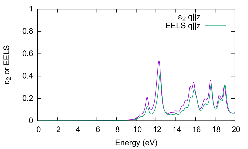
There is little influence of local fields in this case. This is generally the case for semiconductors or materials with a smoothly varying electronic density. We have also shown the EELS spectrum (o-q100.eel_q1_inv_rpa_dyson) for comparison.
LFEs in non-periodic direction
Now let's switch to q perpendicular to the BN plane:
$ yambo -F yambo.in_RPA -V RL -o c -k hartree        and set
...
% LongDrXd
0.000000 | 0.000000 | 1.000000 |        # [Xd] [cc] Electric Field
%
You can try out the default parallel usage now, or run again in serial, i.e.
$ yambo -F yambo.in_RPA  -J q001       (serial)
$ mpirun -np 4 yambo -F yambo.in_RPA  -J q001 &      (parallel, MPI only, 4 tasks)
As noted previously, the log files in parallel appear in the LOG folder, you can follow the execution with tail -F LOG/l-q001_optics_chi_CPU_1 .
Plotting the output file:
$ gnuplot
gnuplot> plot "o-q001.eps_q1_inv_rpa_dyson" u 1:2 w l,"o-q001.eps_q1_inv_rpa_dyson" u 1:4 w l
In this case, the absorption is strongly blueshifted with respect to the in-plane absorption. Furthermore, the influence of local fields is striking, and quenches the spectrum strongly. This is the well known depolarization effect. Local field effects are much stronger in the perpendicular direction because the charge inhomogeneity is dramatic. Many G-vectors are needed to account for the sharp change in the potential across the BN-vacuum interface.
Absorption versus EELS
In order to understand this further, we plot the electron energy loss spectrum for this component and compare with the absorption:
$ gnuplot
$ gnuplot > plot "o-q001.eps_q1_inv_rpa_dyson" w l,"o-q001.eel_q1_inv_rpa_dyson" w l
The conclusion is that the absorption and EELS coincide for isolated systems. To understand why this is, you need to consider the role of the macroscopic screening in the response function and the long-range part of the Coulomb potential. See e.g.[1]
Links
- Back to ICTP 2022#Tutorials
- Back to CECAM VIRTUAL 2021#Tutorials
- ↑ TDDFT from molecules to solids: The role of long‐range interactions, F. Sottile et al, International journal of quantum chemistry 102 (5), 684-701 (2005)
