Real Axis and Lifetimes: Difference between revisions
m (→The materials: Fixing links) |
|||
| (4 intermediate revisions by 2 users not shown) | |||
| Line 8: | Line 8: | ||
In the second section we will use LiF to test the accuracy of the PPA by comparing the results with the real-axis calculation. We will also discuss a non-perturbative solver of the Dyson equation in order to get a more deep insight in the definition of the QP energy and lifetime. | In the second section we will use LiF to test the accuracy of the PPA by comparing the results with the real-axis calculation. We will also discuss a non-perturbative solver of the Dyson equation in order to get a more deep insight in the definition of the QP energy and lifetime. | ||
=The materials = | |||
'''Al''' | '''Al''' | ||
| Line 15: | Line 15: | ||
* Lattice constant 7.50 [a.u.] | * Lattice constant 7.50 [a.u.] | ||
* Plane waves cutoff 16 Hartree (240 RL vectors) | * Plane waves cutoff 16 Hartree (240 RL vectors) | ||
* Al database files: [ | * Al database files: [https://media.yambo-code.eu/educational/tutorials/files/Aluminum.tar.gz Aluminum.tar.gz] | ||
'''LiF''' | '''LiF''' | ||
| Line 22: | Line 22: | ||
* Lattice constant 7.61 [a.u.] | * Lattice constant 7.61 [a.u.] | ||
* Plane waves cutoff 40 Hartree (1800 RL vectors) | * Plane waves cutoff 40 Hartree (1800 RL vectors) | ||
LiF database files: [ | LiF database files: [https://media.yambo-code.eu/educational/tutorials/files/LiF.tar.gz LiF.tar.gz] | ||
= Electronic Lifetimes in Aluminum = | = Electronic Lifetimes in Aluminum = | ||
| Line 39: | Line 39: | ||
The result of the code is the file ''o-01_Lifetimes.qp'' that contains the electronic linewidths. These can be plotted using the columns 3 and 4. | The result of the code is the file ''o-01_Lifetimes.qp'' that contains the electronic linewidths. These can be plotted using the columns 3 and 4. | ||
Now we can perform a quadratic fit of by using a simple gnuplot script | Now we can perform a quadratic fit of by using a simple gnuplot script. | ||
Put the following instructions inside the file ''plot_lifetimes.gnuplot'' | |||
outfile='o-01_Lifetimes.qp' | |||
c(x)=a*x**2 | c(x)=a*x**2 | ||
v(x)=b*x**2 | v(x)=b*x**2 | ||
fit [0:] c(x) | fit [0:] c(x) outfile u 3:4 via a | ||
fit [:0] v(x) | fit [:0] v(x) outfile u 3:4 via b | ||
set ylabel "QP widths [meV]" | set ylabel "QP widths [meV]" | ||
set xlabel "Energy [eV]" | set xlabel "Energy [eV]" | ||
p | p outfile u 3:4 w p t "QP widths" | ||
rep [0:] c(x) t "quadratic fit (conduction)" | rep [0:] c(x) t "quadratic fit (conduction)" | ||
rep [:0] v(x) t "quadratic fit (valence)" | rep [:0] v(x) t "quadratic fit (valence)" | ||
enter gnuplot and load the scrip | |||
$ gnuplot | |||
gnuplot> load "plot_lifetimes.gnuplot" | |||
The result is displayed in the following picture: | The result is displayed in the following picture: | ||
| Line 92: | Line 96: | ||
<span id="08"></span> | <span id="08"></span> | ||
== | == QPs in real-axis GW (Newton solver) (yambo -g n -d -k hartree) == | ||
We can now go beyond the PPA by removing the '''-p p''' command line option. The calculation can be done by using | We can now go beyond the PPA by removing the '''-p p''' command line option. The calculation can be done by using | ||
| Line 103: | Line 107: | ||
[[File:PPA vs RA Z.png]] | [[File:PPA vs RA Z.png]] | ||
== | == QPs in real-axis GW (Secant solver) (yambo -g s -d -k hartree) == | ||
The QP equation is a non-linear equation whose solution must be found using a suitable numerical algorithm. The mostly used, based on the linearization of the self-energy operator is the Newton method. Yambo can also perform a search of the QP energies using a non-linear iterative method based on the '''Secant iterative method'''. | The QP equation is a non-linear equation whose solution must be found using a suitable numerical algorithm. The mostly used, based on the linearization of the self-energy operator is the Newton method. Yambo can also perform a search of the QP energies using a non-linear iterative method based on the '''Secant iterative method'''. | ||
| Line 137: | Line 141: | ||
<span id="11"></span> | <span id="11"></span> | ||
== | == The frequency dependent Green's functions (yambo -g g -d -k hartree) == | ||
By typing | By typing | ||
| Line 147: | Line 151: | ||
From the plot of the imaginary part of the self-energy we see that it correctly changes sign at the Fermi level. We also notice that the self-energy spectral function is characterized by a series of poles far away from the Fermi level. As a consequence the real part of the self-energy is dominated by the frequency dependence of the Hilbert transformation. This frequency dependence, together with the position of the poles, instead, explains the success of the PPA. | From the plot of the imaginary part of the self-energy we see that it correctly changes sign at the Fermi level. We also notice that the self-energy spectral function is characterized by a series of poles far away from the Fermi level. As a consequence the real part of the self-energy is dominated by the frequency dependence of the Hilbert transformation. This frequency dependence, together with the position of the poles, instead, explains the success of the PPA. | ||
== Exercises == | |||
* Confirm the QP energy found with the secant solver by finding "by hand" the QP energy using the plot of the self-energy | * Confirm the QP energy found with the secant solver by finding "by hand" the QP energy using the plot of the self-energy | ||
* What would be (approximatively) the energy dependence of the self-energy in the PPA compared with the full calculation ? | * What would be (approximatively) the energy dependence of the self-energy in the PPA compared with the full calculation ? | ||
Latest revision as of 11:37, 26 September 2024
Introduction
The Plasmon-Pole Approximation (PPA) is a quite robust and useful approach to tackle the QP properties of complex materials. To understand the reasons that are behind the PPA success and to predict the cases where the PPA is expected to fail this tutorial describes how to perform a GW calculation on the real frequency axis.
The tutorial is split in two sections. In the first part we will calculate the electronic lifetimes in bulk aluminium. We will investigate the energy dependence of the lifetimes and their interpretation in terms of a Fermi-liquid theory.
In the second section we will use LiF to test the accuracy of the PPA by comparing the results with the real-axis calculation. We will also discuss a non-perturbative solver of the Dyson equation in order to get a more deep insight in the definition of the QP energy and lifetime.
The materials
Al
- Cubic lattice
- One atom per cell (3 electrons)
- Lattice constant 7.50 [a.u.]
- Plane waves cutoff 16 Hartree (240 RL vectors)
- Al database files: Aluminum.tar.gz
LiF
- FCC lattice
- Two atoms per cell, Li and F (8 electrons)
- Lattice constant 7.61 [a.u.]
- Plane waves cutoff 40 Hartree (1800 RL vectors)
LiF database files: LiF.tar.gz
Electronic Lifetimes in Aluminum
We start from the simple case of bulk aluminum (Al). Al is a metal with a jellium-like band structure. It can be used as a perfect test system to compare the GW results with the analytic expressions we know from the Many-Body Perturbation Theory textbooks.
In order to perform a GW calculation of the electronic linewidths in Al we move in the Al directory
$ cd YAMBO_TUTORIALS/Aluminum
Then we enter in the Yambo folder where a set of pre-calculated core databases is provided and launch yambo without arguments to do a setup run
$ cd Yambo/
$ yambo
The Yambo input file need to calculate the Al linewidths can be found in Inputs/01_Lifetimes. This input file can be used straight away or reproduced using the command
$ yambo -l
At this point we can run the code by using, in the case the existing input file is used
$ yambo -F Inputs/01_Lifetimes -J 01_Lifetimes
The result of the code is the file o-01_Lifetimes.qp that contains the electronic linewidths. These can be plotted using the columns 3 and 4.
Now we can perform a quadratic fit of by using a simple gnuplot script. Put the following instructions inside the file plot_lifetimes.gnuplot
outfile='o-01_Lifetimes.qp'
c(x)=a*x**2
v(x)=b*x**2
fit [0:] c(x) outfile u 3:4  via a
fit [:0] v(x) outfile u 3:4  via b
set ylabel "QP widths [meV]"
set xlabel "Energy  [eV]"
p outfile u 3:4 w p t "QP widths"
rep [0:] c(x) t "quadratic fit (conduction)"
rep [:0] v(x) t "quadratic fit (valence)"
enter gnuplot and load the scrip
$ gnuplot
gnuplot> load "plot_lifetimes.gnuplot"
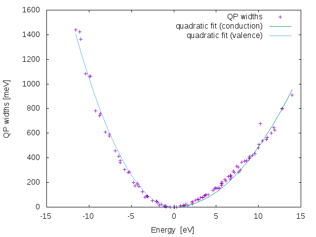
The result is displayed in the following picture:
To understand the physical basis of the GW linewidths we first observe that the general behavior is correct. The linewidths change sign at the chemical potential (set to zero in the code). Moreover by performing a quadratic fit it is easy to see that the linewidths grow quadratically as a function of the distance from the Fermi level.
Beyond the Plasmon-Pole approximation in LiF
In this section we use LiF to perform calculations beyond the PPA in order to understand the limitations of the PPA. The LiF databases are also used in the LiF tutorial, and therefore to avoid confusion we will number the input files starting from the last input of that tutorial.
QPs in the PPA
To run this example we enter the LiF directory
cd YAMBO_TUTORIALS/LiF/GW
We will use the pre-prepared input files in the Inputs folder and thus run the code by using
$ yambo -F Inputs/02_QP_PPA -J PPA
(Note that this input file could be generated using yambo -d -k hartree -g n -p p).
As a result of this run we will find a o-PPA.qp file containing QP corrections and other useful information, such as the renormalization factor Z, the correlation self-energy calculated on-mass shell and the HF self-energy. A section of the o-PPA.qp is reported in the following
#  K-point    Band       Eo         Eqp        E-Eo       LDA        HF         Sc(Eo)     Sc(Eqp)    Sc`(Eo)    Z        Width[meV]  Width[fs]
#
   1.00000    3.00000    0.00000   -2.78101   -2.78101  -22.71824  -30.24829    4.21262    4.74904   -0.19288    0.83831   17.26647   38.12081
   1.00000    4.00000    0.00000   -2.77990   -2.77990  -22.71824  -30.24824    4.21402    4.75009   -0.19283    0.83834   17.26712   38.11938
   1.00000    5.00000    9.00799   10.89507    1.88708  -11.07164   -5.98808   -2.96401   -3.19648   -0.12319    0.89032  -10.51030  -62.62542
   1.00000    6.00000   19.90535   22.26972    2.36438   -8.85663   -2.74568   -3.43248   -3.74658   -0.13285    0.88273   -9.10827  -72.26533
#
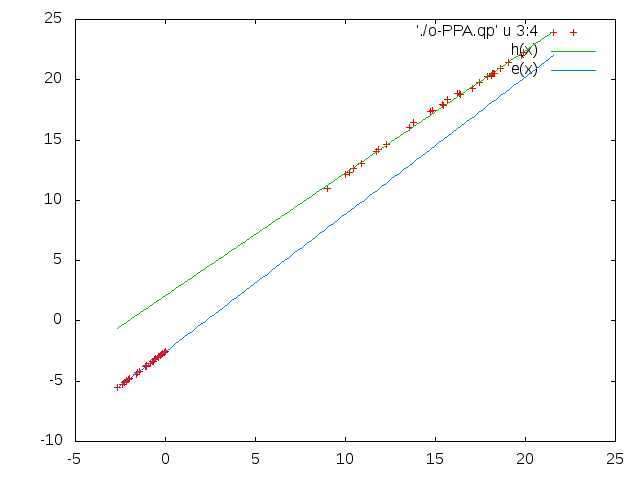
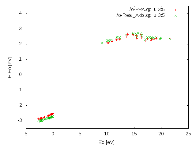
By plotting some of the o-PPA.qp columns it is possible to discuss some physical properties of the LiF QPs. Using columns 3 and 4 we can deduce the band gap renormalization and the stretching of the conduction/valence bands
By adapting the gnuplot fit procedure used before now perform a linear fit of the positive and negative energy dependence of the QP energies to find the gap renormalization and the bands stretching
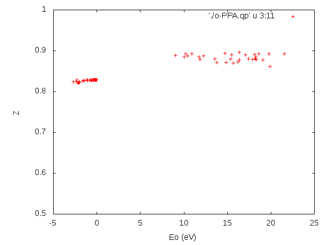
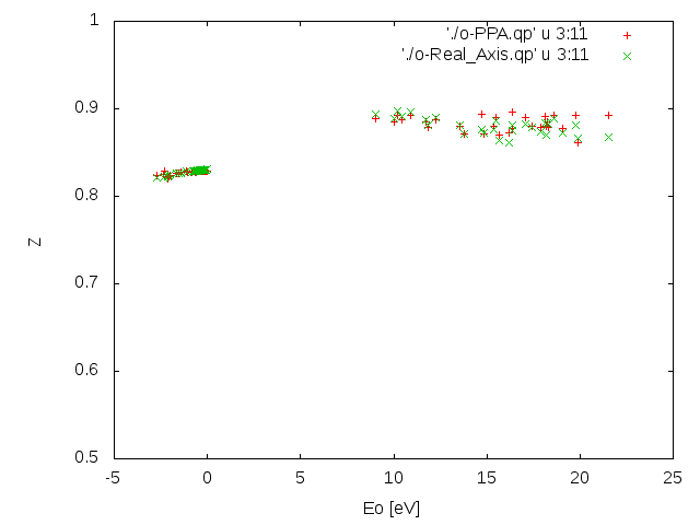
Using columns 3 versus 11 we can plot the renormalization factors. From the quite high mean value (around 0.9) we can infer that LiF is, indeed, a weakly correlated material.
Another crucial consequence of the relatively high renormalization factors is that they point to a possible good performance of the PPA, in this case.
QPs in real-axis GW (Newton solver) (yambo -g n -d -k hartree)
We can now go beyond the PPA by removing the -p p command line option. The calculation can be done by using
localhost:>yambo -F Inputs/03_real_axis -J Real_Axis
In this case Yambo needs to calculate the response function on a large energy range. The number of frequencies, therefore, is much larger then in the case of the PPA. As a consequence the calculation is more cumbersome and long. At the end of the run we can directly compare the results with the PPA case. In particular we can compare the columns 3:5 and the columns 3:11.
QPs in real-axis GW (Secant solver) (yambo -g s -d -k hartree)
The QP equation is a non-linear equation whose solution must be found using a suitable numerical algorithm. The mostly used, based on the linearization of the self-energy operator is the Newton method. Yambo can also perform a search of the QP energies using a non-linear iterative method based on the Secant iterative method.
![]() In numerical analysis, the secant method is a root-finding algorithm that uses a succession of roots of secant lines to better approximate a root of a function f. The secant method can be thought of as a finite difference approximation of Newton's method. However, the method was developed independent of Newton's method. The equation that defines the secant method is:
In numerical analysis, the secant method is a root-finding algorithm that uses a succession of roots of secant lines to better approximate a root of a function f. The secant method can be thought of as a finite difference approximation of Newton's method. However, the method was developed independent of Newton's method. The equation that defines the secant method is:
![]() The first two iterations of the secant method are shown in the following picture. The red curve shows the function f and the blue lines are the secants.
The first two iterations of the secant method are shown in the following picture. The red curve shows the function f and the blue lines are the secants.
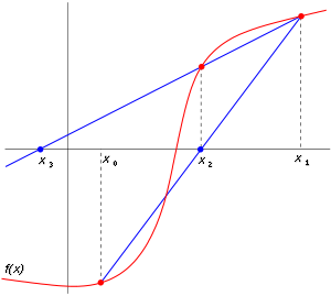
localhost:>yambo -F Inputs/04_real_axis_secant -J Real_Axis
To see if there is any non-linear effect in the solution of the Dyson equation we compare the result of the calculation using the Newton solver with the present case.
Newton solver
#
#  K-point    Band       Eo         Eqp        E-Eo       LDA        HF          Sc(Eo)     Sc(Eqp)    Sc`(Eo)    Z          Width[meV] Width[fs]
#
   1.00000    3.00000    0.00000   -2.98562   -2.98562  -22.71824  -30.24829    3.97144    4.54443   -0.19191    0.83899   18.25441   36.05768
   1.00000    4.00000    0.00000   -2.98467   -2.98467  -22.71824  -30.24824    3.97259    4.54532   -0.19188    0.83901   18.25575   36.05503
   1.00000    5.00000    9.00799   11.03991    2.03192  -11.07164   -5.98808   -2.81392   -3.05165   -0.11699    0.89526  -10.40295  -63.27164
   1.00000    6.00000   19.90535   22.29816    2.39282   -8.85663   -2.74568   -3.34875   -3.71813   -0.15412    0.86636  -48.15936  -13.66737
#
Secant solver
#
#  K-point    Band       Eo         Eqp        E-Eo       LDA        HF          Sc(Eo)     Sc(Eqp)    Sc`(Eo)      Z      Width[meV] Width[fs]
#
   1.00000    3.00000    0.00000   -2.91498   -2.91498  -22.71824  -30.24829    4.61509    5.35346   -0.25328    0.79790   18.47852   35.62038
   1.00000    4.00000    0.00000   -2.91409   -2.91409  -22.71824  -30.24824    4.61592    5.35333   -0.25303    0.79806   18.48304   35.61166
   1.00000    5.00000    9.00799   11.02355    2.01556  -11.07164   -5.98808   -3.06799   -3.34492   -0.13739    0.87921  -10.47416  -62.84146
   1.00000    6.00000   19.90535   22.25859    2.35324   -8.85663   -2.74568   -3.75771   -4.19304   -0.18327    0.84370  -83.27873   -7.90372
#
From the comparison we see that the effect is of the order of 50-60 meV, of the same order of magnitude of the accuracy of the GW calculations.
The frequency dependent Green's functions (yambo -g g -d -k hartree)
By typing
localhost:>yambo -F Inputs/05_rx_greenfunc -J Real_Axis
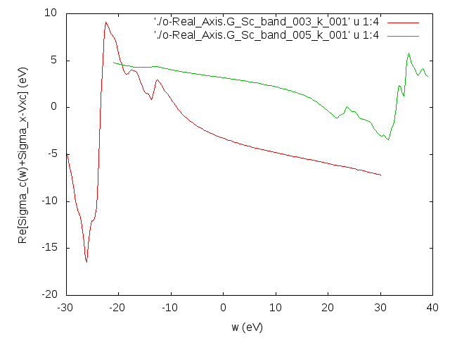
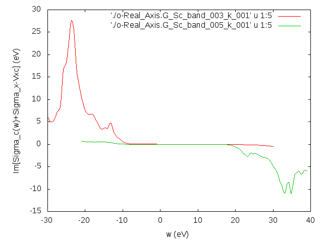
Yambo will calculate the full frequency dependent Green's functions. These will allow us to see what is the real frequency dependence of the self-energy for occupied/empty states.
From the plot of the imaginary part of the self-energy we see that it correctly changes sign at the Fermi level. We also notice that the self-energy spectral function is characterized by a series of poles far away from the Fermi level. As a consequence the real part of the self-energy is dominated by the frequency dependence of the Hilbert transformation. This frequency dependence, together with the position of the poles, instead, explains the success of the PPA.
Exercises
- Confirm the QP energy found with the secant solver by finding "by hand" the QP energy using the plot of the self-energy
- What would be (approximatively) the energy dependence of the self-energy in the PPA compared with the full calculation ?
