Hydrogen chain: Difference between revisions
No edit summary |
m (→Prerequisites: Link fixed) |
||
| (14 intermediate revisions by 2 users not shown) | |||
| Line 1: | Line 1: | ||
In this tutorial you will learn why ALDA fails in extended systems as well as general strategies for treating 1D systems. | In this tutorial you will learn why ALDA fails in extended systems as well as general strategies for treating 1D systems. | ||
== Background == | == Background == | ||
| Line 15: | Line 10: | ||
== Prerequisites == | == Prerequisites == | ||
* The <code>SAVE</code> databases for the hydrogen chain: [http://media.yambo-code.eu/educational/tutorials/files/Hydrogen_Chain.tar.gz Hydrogen_Chain.tar.gz] | |||
* The <code>SAVE</code> databases for the hydrogen chain: [http:// | |||
* The <code>yambo</code> and <code>ypp</code> executables | * The <code>yambo</code> and <code>ypp</code> executables | ||
* <code>gnuplot</code> and [http://www.xcrysden.org <code>xcrysden</code>], for plotting spectra and electron densities | * <code>gnuplot</code> and [http://www.xcrysden.org <code>xcrysden</code>], for plotting spectra and electron densities | ||
| Line 25: | Line 16: | ||
== Failure of the ALDA == | == Failure of the ALDA == | ||
After having downloaded the database files you should have six folders corresponding to the six values of X (2.05, 2.1, 2.2., 2.3, 2.4 and 2.5). | After having downloaded the database files you should have six folders corresponding to the six values of X (2.05, 2.1, 2.2., 2.3, 2.4 and 2.5). | ||
$ cd YAMBO_TUTORIALS/Hydrogen_Chain/ | |||
$ ls | |||
ABINIT/ Inputs/ YAMBO/ | |||
The first step of this tutorial is to run the calculation of the dynamical absorption in the TDLDA approximation. | The first step of this tutorial is to run the calculation of the dynamical absorption in the TDLDA approximation. | ||
We will describe here only the case of X=2.05 a.u. You are invited to repeat the calculation for X=2.5 and, if you wish, for all the other cases. | We will describe here only the case of X=2.05 a.u. You are invited to repeat the calculation for X=2.5 and, if you wish, for all the other cases. | ||
Enter the 2.05 directory and run the initialization step | Enter the 2.05 directory and run the initialization step | ||
$ cd 2.05 | $ cd YAMBO/2.05 | ||
$ ls | $ ls | ||
BSE/ SAVE/ | BSE/ SAVE/ | ||
$ yambo ''(initialization)'' | $ yambo ''(initialization)'' | ||
From reading the r_setup file we notice that the system has a small (0.27 eV) gap. Now generate the input file for the TDLDA calculation by typing | |||
$ yambo -o b - | From reading the ''r_setup'' file we notice that the system has a small (0.27 eV) gap. Now generate the input file for the TDLDA calculation by typing | ||
$ yambo -o b -k alda -y d -V qp -F in_alda | |||
and change the highlighted lines in the input file: | and change the highlighted lines in the input file: | ||
optics # [R OPT] Optics | optics # [R OPT] Optics | ||
bse # [R BSK] Bethe Salpeter Equation. | bse # [R BSK] Bethe Salpeter Equation. | ||
| Line 49: | Line 47: | ||
BEnSteps= '''1000''' # [BSS] Energy steps | BEnSteps= '''1000''' # [BSS] Energy steps | ||
Now use the ''resp'' verbosity to activate the flag needed to dump to file the eigenvectors of the BS Hamiltonian | Now use the ''resp'' verbosity to activate the flag needed to dump to file the eigenvectors of the BS Hamiltonian | ||
$ yambo -o b -t a -y d -V resp | |||
$ yambo -o b -t a -y d -V resp -F in_alda | |||
and remove the ''#'' from the appropriate flag to activate the option: | and remove the ''#'' from the appropriate flag to activate the option: | ||
#WRbsWF # [BSS] Write to disk excitonic the FWs | #WRbsWF # [BSS] Write to disk excitonic the FWs | ||
Now run yambo | |||
Now run yambo | |||
$ yambo -F in_alda -J ALDA | |||
In the folder ./BSE you will find the absorption spectra (''o-BSE_RIM.eps_q001-bd'') calculated using the Many-Body based Bethe-Salpeter(BS) equation. We will keep the results of the Bethe-Salpeter equation as a reference for our calculations. The BS equation leads indeed a proper and accurate description of the optical properties of the H<sub>2</sub> molecular chains.<br /> | |||
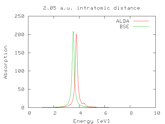
If you plot the ALDA result against the BS one you will find that there is a reasonable agreement between the two curves. | If you plot the ALDA result against the BS one you will find that there is a reasonable agreement between the two curves. | ||
| Line 61: | Line 68: | ||
$ cd ../2.5 | $ cd ../2.5 | ||
$ yambo | $ yambo | ||
$ yambo -o b -t a -y d -V resp | $ yambo -o b -t a -y d -V resp -F in_alda | ||
modify the input file and run again <code>yambo</code>. | |||
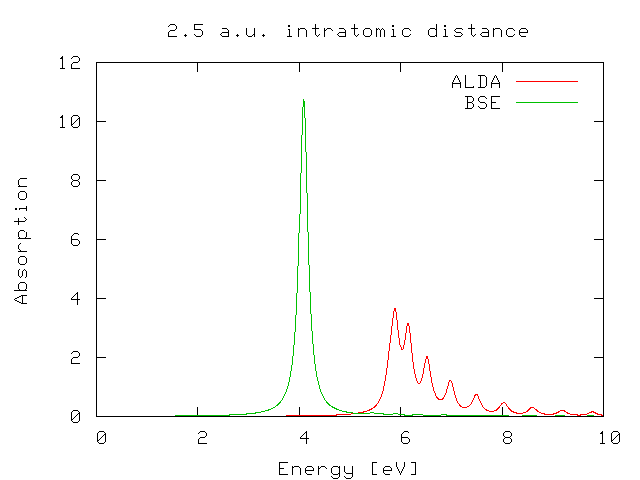
If you plot again the ALDA result against the BS one you will find that in this case the performance of the ALDA is much worse. | If you plot again the ALDA result against the BS one you will find that in this case the performance of the ALDA is much worse. | ||
| Line 77: | Line 87: | ||
To this end we can use the yambo post/pre processor (YPP). <code>ypp</code> is capable of performing some basic analyses using the pre-calculated informations stored in the yambo databases.<br /> | To this end we can use the yambo post/pre processor (YPP). <code>ypp</code> is capable of performing some basic analyses using the pre-calculated informations stored in the yambo databases.<br /> | ||
YPP works like yambo. It uses a series of options to create an input file containing only the variables that are relevant to that type of calculation. Launch it with the help (-H) flag to see a full list of options. | YPP works like yambo. It uses a series of options to create an input file containing only the variables that are relevant to that type of calculation. Launch it with the help (-H) flag to see a full list of options. | ||
$ cd 2.05/ | $ cd 2.05/ | ||
$ ypp -H | $ ypp -H | ||
To plot the density we need to type | To plot the density we need to type | ||
ypp - | |||
The input file '' | $ ypp -s d -F in_density | ||
The input file ''in_density'' will be | |||
Format= | |||
electrons # [R] Electrons (and holes) | |||
FFTGvecs= 7659 | density # [R] Density | ||
Format= "g" # Output format [(c)ube/(g)nuplot/(x)crysden] | |||
Direction= "1" # [rlu] [1/2/3] for 1d or [12/13/23] for 2d [123] for 3D | |||
FFTGvecs= 7659 RL # [FFT] Plane-waves | |||
As our system is one-dimensional and it is lying parallel to the z axis we need to change to ''Direction="12"'' so to perform a contour plot on the "XY" plane. | As our system is one-dimensional and it is lying parallel to the z axis we need to change to ''Direction="12"'' so to perform a contour plot on the "XY" plane. | ||
To use XCrysden switch to "x" the value of the ''Format'' variable.<br /> | To use XCrysden switch to "x" the value of the ''Format'' variable.<br /> | ||
Now you can launch ypp. | Now you can launch ypp. | ||
$ ypp | |||
At the end of the quick calculation you will find in your directory the file ''o.density_2d.xsf'' that you can plot using Xcrysden. You can view the density directly using the | $ ypp -F in_density | ||
$ | |||
At the end of the quick calculation you will find in your directory the file ''o.density_2d.xsf'' that you can plot using Xcrysden. | |||
You can view the density directly using the [[Bash_scripts|launch_xcrysden.sh]] shell script. To use it type: | |||
$ launch_xcrysden.sh o.density_2d.xsf | |||
Follow the same procedure for the other distance and compare the two densities. You should see something like | Follow the same procedure for the other distance and compare the two densities. You should see something like | ||
[[File:Chain 2.05 structure.png|300px]] [[File:Chain_2.5.png|300px]] <br> | [[File:Chain 2.05 structure.png|300px]] [[File:Chain_2.5.png|300px]] <br> | ||
| Line 110: | Line 128: | ||
A mean large distance between the electron and hole also reflects the poor correlation felt by the two bodies. YPP can plot either the case where the electron and the hole are forced to be in the same space point, or the case where the hole's position is fixed somewhere and the electron is left free to move. This second case is more appropriate here.<br /> | A mean large distance between the electron and hole also reflects the poor correlation felt by the two bodies. YPP can plot either the case where the electron and the hole are forced to be in the same space point, or the case where the hole's position is fixed somewhere and the electron is left free to move. This second case is more appropriate here.<br /> | ||
We need first to identify the index of the corresponding eigenstate. Running | We need first to identify the index of the corresponding eigenstate. Running | ||
$ ypp -e s | |||
YPP will create a file named ''o.exc_I_sorted'' that contains the list of peaks in the dielectric function ordered with increasing peak intensity. | $ ypp -e s -J ALDA | ||
# E [ev] Strength Index | YPP will create a file named ''o-ALDA.exc_I_sorted'' that contains the list of peaks in the dielectric function ordered with increasing peak intensity. | ||
# | |||
# | |||
# E [ev] Strength Index | |||
# | |||
3.783688 1.000000 1.000000 | 3.783688 1.000000 1.000000 | ||
4.38457 0.03179 3.00000 | 4.38457 0.03179 3.00000 | ||
5.171 0.3731E-2 5.000< | 5.171 0.3731E-2 5.000< | ||
We see that the peak with energy 3.78 dominates the spectra and it corresponds to the index 1. If we type now | We see that the peak with energy 3.78 dominates the spectra and it corresponds to the index 1. If we type now | ||
$ ypp -e w | |||
$ ypp -e w -F in_tdlda_density | |||
to get the input file | to get the input file | ||
exc_wf # [R] Excitonic Wavefunction | exc_wf # [R] Excitonic Wavefunction | ||
excp # [R] Excitonic Properties | excp # [R] Excitonic Properties | ||
| Line 135: | Line 160: | ||
0.000 | 0.000 | 0.000 | # [cc] Hole position in unit cell | 0.000 | 0.000 | 0.000 | # [cc] Hole position in unit cell | ||
% | % | ||
It is interesting to do a 3D plot. To this end we set ''Direction="123"'' and replace the first component in Cells with 16 (this value will expand the unit cell along the X direction). The ''States'' variable is already set to the peak number 1.<br /> | It is interesting to do a 3D plot. To this end we set ''Direction="123"'' and replace the first component in Cells with 16 (this value will expand the unit cell along the X direction). The ''States'' variable is already set to the peak number 1.<br /> | ||
We put the hole in the middle of the chain by setting | We put the hole in the middle of the chain by setting | ||
% Hole | % Hole | ||
1.02500 | 12.50000 | 12.50000 | # [cc] Hole position in unit ce | 1.02500 | 12.50000 | 12.50000 | # [cc] Hole position in unit ce | ||
% | % | ||
Remember that the first field '''must be set to the interatomic distance divided by two'''. In the case of 2.5 a.u. the first field will be 1.25.<br /> | Remember that the first field '''must be set to the interatomic distance divided by two'''. In the case of 2.5 a.u. the first field will be 1.25.<br /> | ||
If we run now ypp | If we run now ypp | ||
$ | |||
$ ypp -F in_tdlda_density -J ALDA | |||
'''remembering to put the ALDA jobstring to allow Yambo to find the ALDA databases'''. This will create the file ''o-ALDA.exc_3d_1.xsf'' that you can plot by using | |||
$ launch_xcrysden.sh o-ALDA.exc_3d_1.xsf | |||
If we compare the plot with the one obtained by solving the BS equation we should see | If we compare the plot with the one obtained by solving the BS equation we should see | ||
{| class="wikitable" style="text-align: center; | {| class="wikitable" style="text-align: center; | ||
|colspan="2"|'''Excitation wavefunctions for 2.05 a.u. distance''' | |colspan="2"|'''Excitation wavefunctions for 2.05 a.u. distance''' | ||
| Line 173: | Line 209: | ||
The key point is to realize that, indeed, the f<sub>xc</sub> kernel acts like a self-energy in the Dyson equation for χ. As in the case of quasiparticles, the most optimal self-energy can be chosen by looking at the structure of the bare propagator, χ<sub>0</sub> in this case.<br /> | The key point is to realize that, indeed, the f<sub>xc</sub> kernel acts like a self-energy in the Dyson equation for χ. As in the case of quasiparticles, the most optimal self-energy can be chosen by looking at the structure of the bare propagator, χ<sub>0</sub> in this case.<br /> | ||
In the long wavelength limit χ<sub>0</sub> behaves like q<sup>2</sup>. As a naive consequence the self-energy must cancel this power dependence to ensure that the product f<sub>xc</sub>χ<sub>0</sub> remains finite in the optical limit. | In the long wavelength limit χ<sub>0</sub> behaves like q<sup>2</sup>. As a naive consequence the self-energy must cancel this power dependence to ensure that the product f<sub>xc</sub>χ<sub>0</sub> remains finite in the optical limit. | ||
This simple argument is enough to introduce the long-range TDDFT kernel:<br> | This simple argument is enough to introduce the long-range TDDFT kernel:<br> | ||
[[File:Chain_PIC_doc_TDDFT-129.png]] <br> | [[File:Chain_PIC_doc_TDDFT-129.png]] <br> | ||
Now we will use this kernel with a static approximation for the parameter alpha, first for the chain of intermolecular distance 2.5 a.u.. | Now we will use this kernel with a static approximation for the parameter alpha, first for the chain of intermolecular distance 2.5 a.u.. | ||
Enter the 2.5 directory and generate the input file for a TDDFT calculation in reciprocal space, specifying you want the long-range kernel: | Enter the 2.5 directory and generate the input file for a TDDFT calculation in reciprocal space, specifying you want the long-range kernel: | ||
$ cd 2.5 | $ cd 2.5 | ||
$ yambo -o c - | $ yambo -o c -k lrc -F in_LRC | ||
Change the highlighted variables in the input file: | Change the highlighted variables in the input file: | ||
Chimod= "LRC" # [X] IP/Hartree/ALDA/LRC/BSfxc | Chimod= "LRC" # [X] IP/Hartree/ALDA/LRC/BSfxc | ||
LRC_alpha= '''0.000000''' # [TDDFT] LRC alpha factor | LRC_alpha= '''0.000000''' # [TDDFT] LRC alpha factor | ||
| Line 193: | Line 235: | ||
NGsBlkXd= '''100''' RL # [Xd] Response block size (Put some local fields, not too much) | NGsBlkXd= '''100''' RL # [Xd] Response block size (Put some local fields, not too much) | ||
ETStpsXd= '''1000''' # [Xd] Total Energy steps | ETStpsXd= '''1000''' # [Xd] Total Energy steps | ||
and run yambo. Now we can perform different calculations assigning different values to the variable LRC_alpha. This value is a static approximation to α(ω) in the long-range expression for f<sub>xc</sub>. This must be negative (the interaction between electron and hole is attractive). Try different numbers in the range 0 to -20. You will see that around <code>LRC_alpha=-19</code> we obtain the same excitation energy of the BSE spectrum:<br> | and run yambo. Now we can perform different calculations assigning different values to the variable LRC_alpha. This value is a static approximation to α(ω) in the long-range expression for f<sub>xc</sub>. This must be negative (the interaction between electron and hole is attractive). Try different numbers in the range 0 to -20. You will see that around <code>LRC_alpha=-19</code> we obtain the same excitation energy of the BSE spectrum:<br> | ||
[[File:Chain lrc.png]] <br> | [[File:Chain lrc.png]] <br> | ||
Now you can repeat the same calculations for the chain with 2.05 intermolecular distance. Once you will find the optimal value of %alpha, you will realize that as expected, it is one order of magnitude smaller than the one needed for the previous, more inhomogeneous system. | Now you can repeat the same calculations for the chain with 2.05 intermolecular distance. Once you will find the optimal value of %alpha, you will realize that as expected, it is one order of magnitude smaller than the one needed for the previous, more inhomogeneous system. | ||
[[File:Chain lrc 2.png]] <br> | [[File:Chain lrc 2.png]] <br> | ||
To conclude this tutorial note that the value of &alpha you found is much larger then in any solid, as showed in this picture. Can you understand why? <br /> | To conclude this tutorial note that the value of &alpha you found is much larger then in any solid, as showed in this picture. Can you understand why? <br /> | ||
[[File:Chain alpha.png]] | [[File:Chain alpha.png]] | ||
= | = The Bethe-Salpeter Equation applied to 1D systems = | ||
The H<sub>2</sub> hydrogen chain constitutes an example of a perfectly one-dimensional system. | The H<sub>2</sub> hydrogen chain constitutes an example of a perfectly one-dimensional system. | ||
This property causes some tricky numerical problems that are, however, related to a precise physical process: the extreme confinement of 3D electrons in a small region of space. | This property causes some tricky numerical problems that are, however, related to a precise physical process: the extreme confinement of 3D electrons in a small region of space. | ||
If we use yambo to perform a BS calculation you will immediately see where the problem is! | If we use yambo to perform a BS calculation you will immediately see where the problem is! | ||
'''Let's move in the 2.5 folder''' | |||
$ cd YAMBO_TUTORIALS/Hydrogen_Chain/YAMBO/2.5 | |||
We start by generating the input file. At the command line we have to tell yambo to construct the BSE <code>(-o b)</code> , to calculate the static screened interaction <code>(-b)</code>, and to diagonalize the BS matrix <code>(-y d)</code>, as well as activate a higher verbosity level in the input file <code>-V qp</code>: | We start by generating the input file. At the command line we have to tell yambo to construct the BSE <code>(-o b)</code> , to calculate the static screened interaction <code>(-b)</code>, and to diagonalize the BS matrix <code>(-y d)</code>, as well as activate a higher verbosity level in the input file <code>-V qp</code>: | ||
$ yambo -o b -b -y d -V qp -F in_BSE | |||
The generated input file describes our first attempt to calculate the excitonic polarization spectrum of the H chain. Let's now change the bolded values | |||
BSEmod= '''"causal"''' # [BSE] resonant/causal/coupling | BSEmod= '''"causal"''' # [BSE] resonant/causal/coupling | ||
'''BSENGBlk= 1''' RL # [BSK] Screened interaction block size | |||
BSENGexx= '''7659''' RL # [BSK] Exchange components | BSENGexx= '''7659''' RL # [BSK] Exchange components | ||
% BndsRnXs | % BndsRnXs | ||
1 | '''20''' | # [BSK] Bands range | 1 | '''20''' | # [BSK] Bands range | ||
% | % | ||
NGsBlkXs= 1 RL # [Xs] Response block size | '''NGsBlkXs= 1''' RL # [Xs] Response block size | ||
First we consider only the resonant part of the BS equation: | First we consider only the resonant part of the BS equation: | ||
BSEmod= "resonant" | BSEmod= "resonant" | ||
Second, include a QP gap correction of 3.5 eV | Second, include a QP gap correction of 3.5 eV | ||
% KfnQP_E | % KfnQP_E | ||
3.50000 | 1.000000 | 1.000000 | # [EXTQP BSK BSS] E parameters (c/v) | 3.50000 | 1.000000 | 1.000000 | # [EXTQP BSK BSS] E parameters (c/v) | ||
% | % | ||
Third, decide some reasonable size of the inverse dielectric function that defines the statically screened interaction (normally this has to be determined by convergence studies): | Third, decide some reasonable size of the inverse dielectric function that defines the statically screened interaction (normally this has to be determined by convergence studies): | ||
NGsBlkXs= 111 | NGsBlkXs= 111 | ||
BSENGexx= 111 | BSENGexx= 111 | ||
Fourth, you should change the BSE and polarization function band ranges: | Fourth, you should change the BSE and polarization function band ranges: | ||
% BSEBands | % BSEBands | ||
| Line 280: | Line 292: | ||
1 | 2 | # [Xs] Polarization function bands | 1 | 2 | # [Xs] Polarization function bands | ||
% | % | ||
Two bands are enough in this case to get reasonable results. | Two bands are enough in this case to get reasonable results. | ||
Remember also to uncomment the variable <code>WRbsWF</code> if you want to plot the excitonic wave function afterwords. | |||
< | |||
Finally, we launch yambo | |||
$ yambo -J BSE | |||
and to our great surprise the polarization spectrum we obtain is completely wrong, with just a poor signal around 3eV which is nonsense: | |||
[[File:2.5_bse_no_RIM.png]] | |||
As you can see '''the excitonic peak has even a negative intensity'''! | |||
The reason of this serious failure of the BS calculation is due to the peculiar geometry of the H chain, and of corresponding BZ sampling that is strictly one dimensional. This is readily detected in any report file, like ''r_setup'' | |||
[...] | |||
[02.04] K-grid lattice | |||
==== | ====================== | ||
Compatible Grid is 1D | |||
Compatible Grid | |||
B1 [rlu]= -0.01250 0.00000 0.00000 | B1 [rlu]= -0.01250 0.00000 0.00000 | ||
Grid dimensions | Grid dimensions : 80 | ||
K lattice UC volume [au]: 0.0011 | K lattice UC volume [au]: 0.0011 | ||
As a consequence the ''region'' of space assigned to each k-point is strongly compressed in one of the dimensions, like the thin slices of this picture | As a consequence the ''region'' of space assigned to each k-point is strongly compressed in one of the dimensions, like the thin slices of this picture | ||
[[File:Chain_slices. | [[File:Chain_slices.jpg]] | ||
]]The drastic consequence of this compression is that each region receives a piece of the electron-electron interaction that is multiplied by a ''form factor'' of the region, that, in general '''is assumed spatially constant'''. With such a severe sampling of the BZ this assumption is no longer valid and the screened interaction is anomalously enhanced. | |||
The drastic consequence of this compression is that each region receives a piece of the electron-electron interaction that is multiplied by a ''form factor'' of the region, that, in general '''is assumed spatially constant'''. With such a severe sampling of the BZ this assumption is no longer valid and the screened interaction is anomalously enhanced. | |||
To avoid this anomalous electron-electron interaction we use the Random Integration Method (<code>-c</code> option). | |||
$ yambo -r -o b -b -y d -F in_BSE_RIM | |||
and modify the <code>RandQpts</code> and <code>RandGvec</code> variables: | |||
RandQpts= 1000000 # [RIM] Number of random q-points in the BZ | |||
RandGvec= 1 RL # [RIM] Coulomb interaction RS components | |||
Here ''RandQpts'' specifies the number of random points to use and ''RandGvec'' the number of RL components to evaluate. | |||
After launching | |||
$ yambo -F in_BSE_RIM -J BSE_RIM | |||
we notice a new section in the report file: | |||
we notice a new section in the report file | |||
[04] Coulomb potential Random Integration (RIM) | [04] Coulomb potential Random Integration (RIM) | ||
========= | ========= | ||
| Line 356: | Line 378: | ||
Q [39]: 0.663225 0.981867 * Q [40]: 0.680678 0.983004 | Q [39]: 0.663225 0.981867 * Q [40]: 0.680678 0.983004 | ||
Q [41]: 0.698132 0.984061 | Q [41]: 0.698132 0.984061 | ||
The final BS polarizability is, now, physically correct and substantially different from ALDA. | The interesting result is that the 2<sup>nd</sup> and the 4<sup>th</sup> columns of numbers reflect the effect of the BZ compression: 1 means little effect, small numbers mean large effect. We see that the effect is huge for points in the BZ with small modulus (1<sup>st</sup> and 3<sup>rd</sup> columns). | ||
The final BS polarizability is, now, physically correct and substantially different from ALDA:<br> | |||
[[File:Chain_bse_rim.png|512x384px]] | |||
= <span id="exercises"></span>Additional Exercises = | |||
The H chain is a one dimensional system, and, consequently it should not absorb when the light is polarized perpendicularly to the chain axis (the x direction). | The H chain is a one dimensional system, and, consequently it should not absorb when the light is polarized perpendicularly to the chain axis (the x direction). | ||
# Repeat the | # Repeat the RPA, ALDA, and BSE calculations for light polarized perpendicular to the chain axis to verify that the polarization is much smaller than in the parallel case. | ||
# Use ypp to plot the excitonic wave function. | # Use ypp to plot the excitonic wave function. | ||
# Repeat the whole tutorial for the other | # Repeat the whole tutorial for the other interatomic distances. | ||
Latest revision as of 09:16, 17 November 2023
In this tutorial you will learn why ALDA fails in extended systems as well as general strategies for treating 1D systems.
Background
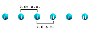
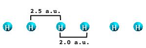
It is well known that the performance of ALDA gradually worsens when moving from 0 to 3 dimensions. Why this happens can be understood by studying a simple system: the infinite H2 molecular chain. This is a very simple physical system consisting of H atoms that are distributed in sets of two atoms placed at a variable distance X from each other. The physical properties of the chain are functions of the distance X. When X=2. a.u. the system is metallic. By increasing X the chain becomes semiconducting with increasing gap.
The conclusions of this tutorial do not mean to be general, but they should convince you that there is a link between the local assumption of the ALDA and the polarization of electrons in extended directions.
Prerequisites
- The
SAVEdatabases for the hydrogen chain: Hydrogen_Chain.tar.gz - The
yamboandyppexecutables gnuplotandxcrysden, for plotting spectra and electron densities
Failure of the ALDA
After having downloaded the database files you should have six folders corresponding to the six values of X (2.05, 2.1, 2.2., 2.3, 2.4 and 2.5).
$ cd YAMBO_TUTORIALS/Hydrogen_Chain/
$ ls
ABINIT/ Inputs/ YAMBO/
The first step of this tutorial is to run the calculation of the dynamical absorption in the TDLDA approximation. We will describe here only the case of X=2.05 a.u. You are invited to repeat the calculation for X=2.5 and, if you wish, for all the other cases.
Enter the 2.05 directory and run the initialization step
$ cd YAMBO/2.05
$ ls
BSE/  SAVE/
$ yambo            (initialization)
From reading the r_setup file we notice that the system has a small (0.27 eV) gap. Now generate the input file for the TDLDA calculation by typing
$ yambo -o b -k alda -y d -V qp -F in_alda
and change the highlighted lines in the input file:
optics                       # [R OPT] Optics
bse                          # [R BSK] Bethe Salpeter Equation.
alda_fxc                     # [R TDDFT] The ALDA TDDFT kernel
bss                          # [R BSS] Bethe Salpeter Equation solver
...
% KfnQP_E
 3.500000 | 1.000000 | 1.000000 |      # [EXTQP BSK BSS] E parameters (c/v)
%
% BSEBands
  1 | 2 |
%
BEnSteps= 1000                # [BSS] Energy steps
Now use the resp verbosity to activate the flag needed to dump to file the eigenvectors of the BS Hamiltonian
$ yambo -o b -t a -y d -V resp -F in_alda
and remove the # from the appropriate flag to activate the option:
#WRbsWF # [BSS] Write to disk excitonic the FWs
Now run yambo
$ yambo -F in_alda -J ALDA
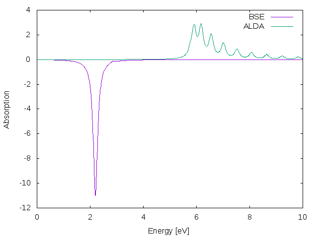
In the folder ./BSE you will find the absorption spectra (o-BSE_RIM.eps_q001-bd) calculated using the Many-Body based Bethe-Salpeter(BS) equation. We will keep the results of the Bethe-Salpeter equation as a reference for our calculations. The BS equation leads indeed a proper and accurate description of the optical properties of the H2 molecular chains.
If you plot the ALDA result against the BS one you will find that there is a reasonable agreement between the two curves.
Now, please, repeat the same procedure in the 2.5 folder
$ cd ../2.5
$ yambo
$ yambo -o b -t a -y d -V resp -F in_alda
modify the input file and run again yambo.
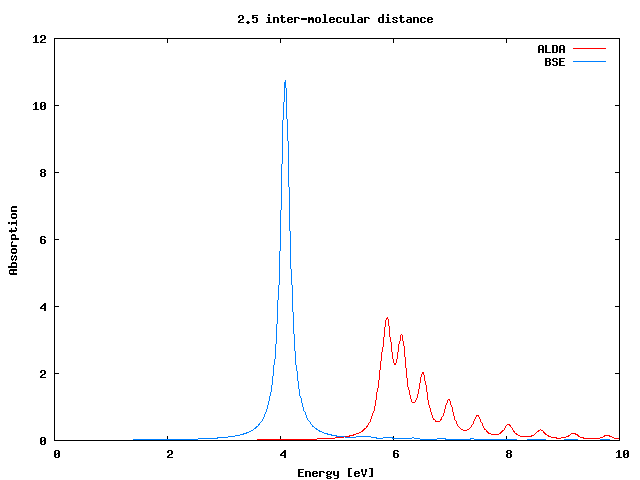
If you plot again the ALDA result against the BS one you will find that in this case the performance of the ALDA is much worse.
The question now is ... why?
A closer look: analysis of the electronic states
At this stage we need to get some more information from the TDLDA calculations that can be compared with the "exact" BS results. Let's proceed by plotting the electronic density and the wavefunction corresponding to the most intense peak in the dynamical polarizability.
The electronic density
The easiest quantity we can compare for the two chains (2.05 and 2.5 intratomic distance) is the electronic density.
To this end we can use the yambo post/pre processor (YPP). ypp is capable of performing some basic analyses using the pre-calculated informations stored in the yambo databases.
YPP works like yambo. It uses a series of options to create an input file containing only the variables that are relevant to that type of calculation. Launch it with the help (-H) flag to see a full list of options.
$ cd 2.05/
$ ypp -H
To plot the density we need to type
$ ypp -s d -F in_density
The input file in_density will be
electrons                      # [R] Electrons (and holes)
density                        # [R] Density
Format= "g"                    # Output format [(c)ube/(g)nuplot/(x)crysden]
Direction= "1"                 # [rlu] [1/2/3] for 1d or [12/13/23] for 2d [123] for 3D
FFTGvecs=  7659        RL      # [FFT] Plane-waves
As our system is one-dimensional and it is lying parallel to the z axis we need to change to Direction="12" so to perform a contour plot on the "XY" plane.
To use XCrysden switch to "x" the value of the Format variable.
Now you can launch ypp.
$ ypp -F in_density
At the end of the quick calculation you will find in your directory the file o.density_2d.xsf that you can plot using Xcrysden.
You can view the density directly using the launch_xcrysden.sh shell script. To use it type:
$ launch_xcrysden.sh o.density_2d.xsf
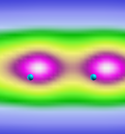
Follow the same procedure for the other distance and compare the two densities. You should see something like
We see that the smaller the gap (@ 2.05 a.u.) the more delocalized the electronic density. The consequence is that electrons can move more freely in the 2.05 case. At the same time, however, the polarization will be more "metallic-like" where the ALDA is expected to work better.
The TDLDA excitations wavefunction
Using YPP we can do something more. We can plot the wavefunction corresponding to the most intense peak in the dielectric function. The excitation wavefunction is a two-coordinate (r1, and r2) function and represents the probability amplitude of finding the electron at position r1 when the hole is in r2. The larger this probability the more delocalized is the perturbation induced by the external field.
A mean large distance between the electron and hole also reflects the poor correlation felt by the two bodies. YPP can plot either the case where the electron and the hole are forced to be in the same space point, or the case where the hole's position is fixed somewhere and the electron is left free to move. This second case is more appropriate here.
We need first to identify the index of the corresponding eigenstate. Running
$ ypp -e s -J ALDA
YPP will create a file named o-ALDA.exc_I_sorted that contains the list of peaks in the dielectric function ordered with increasing peak intensity.
#
#  E [ev]     Strength   Index
#
 3.783688   1.000000   1.000000
  4.38457    0.03179    3.00000
 5.171     0.3731E-2   5.000<
We see that the peak with energy 3.78 dominates the spectra and it corresponds to the index 1. If we type now
$ ypp -e w -F in_tdlda_density
to get the input file
exc_wf                       # [R] Excitonic Wavefunction
excp                         # [R] Excitonic Properties
plot                         # [R] Plot
Format= "x"                  # Output format [(g)nuplot/(x)crysden]
Direction= "12"             # [rlu] [1/2/3] for 1d or [12/13/23] for 2d [123] for 3D
FFTGvecs=  7659          RL  # [FFT] Plane-waves
States= "1 - 1"              # Index of the BS state(s)
Degen_Step=   0.0100     eV  # Maximum energy separation of two degenerate states
% Cells
1 |  1 |  1 |                        # Number of cell repetitions (even or 1)
%
% Hole
 0.000    | 0.000    | 0.000    |      # [cc] Hole position in unit cell
%
It is interesting to do a 3D plot. To this end we set Direction="123" and replace the first component in Cells with 16 (this value will expand the unit cell along the X direction). The States variable is already set to the peak number 1.
We put the hole in the middle of the chain by setting
% Hole
1.02500 | 12.50000 | 12.50000  |           # [cc] Hole position in unit ce
%
Remember that the first field must be set to the interatomic distance divided by two. In the case of 2.5 a.u. the first field will be 1.25.
If we run now ypp
$ ypp -F in_tdlda_density -J ALDA
remembering to put the ALDA jobstring to allow Yambo to find the ALDA databases. This will create the file o-ALDA.exc_3d_1.xsf that you can plot by using
$ launch_xcrysden.sh o-ALDA.exc_3d_1.xsf
If we compare the plot with the one obtained by solving the BS equation we should see
| Excitation wavefunctions for 2.05 a.u. distance | |

|
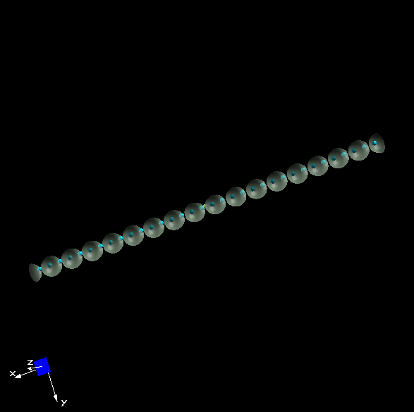
|
| BS equation | TDLDA |
| Excitation wavefunctions for 2.5 a.u. distance | |
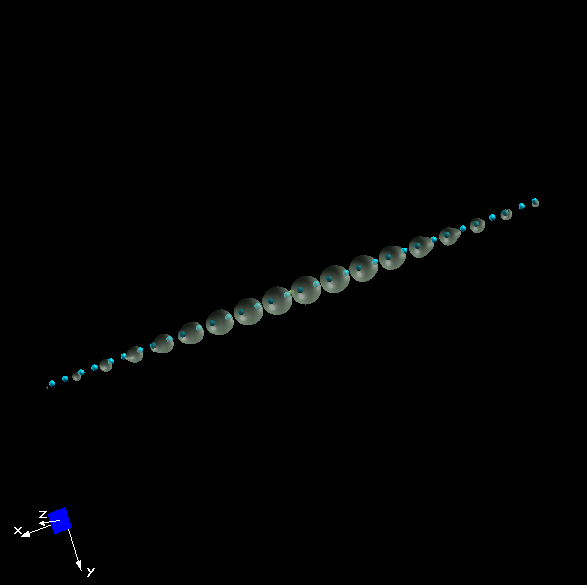
|
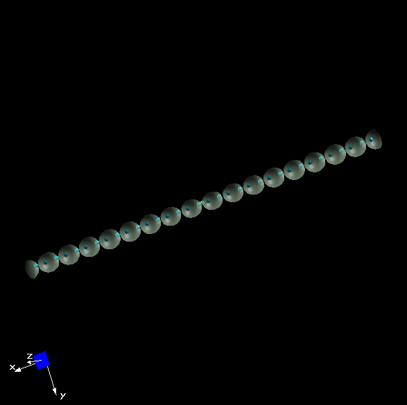
|
| BS equation | TDLDA |
We immediately see that, while the ALDA excitation is always spread all over the chain, in the 2.5 distance case the "true" wavefunction acquires a tail that decreases the probability of finding the electron and the hole very far from each other.
This saturation of the excitation wavefunction is the physical reason for the poor performance of the ALDA. As it is a local approximation it cannot take into account a long-range correlation between the electron and the hole.
A long-range kernel beyond the TDLDA
So, we realized the a simple plot of the excitation wavefunction can pin down the possible reasons for the breakdown of the ALDA. In general if you know the problem, you should be half way through the quest for a solution. Is it true?
We have seen the failure of the ALDA in the case of the H2 chain when the intra-molecular distance increases. We also have seen how the excitation wave function differs from the one obtained by solving the Bethe Salpeter equation in the case of 2.5 a.u. intermolecular distance. Such discrepancy has been traced back to the the long-range correlation between the electron and hole, that cannot be captured by the simple local approximation.
Now, we use yambo to check whether simple approximations for the fxc kernel can cure the ALDA drawbacks. To this end we use the Reciprocal space Dyson equation for the response function, activated using the yambo -o c option.
The key point is to realize that, indeed, the fxc kernel acts like a self-energy in the Dyson equation for χ. As in the case of quasiparticles, the most optimal self-energy can be chosen by looking at the structure of the bare propagator, χ0 in this case.
In the long wavelength limit χ0 behaves like q2. As a naive consequence the self-energy must cancel this power dependence to ensure that the product fxcχ0 remains finite in the optical limit.
This simple argument is enough to introduce the long-range TDDFT kernel:
Now we will use this kernel with a static approximation for the parameter alpha, first for the chain of intermolecular distance 2.5 a.u.. Enter the 2.5 directory and generate the input file for a TDDFT calculation in reciprocal space, specifying you want the long-range kernel:
$ cd 2.5
$ yambo -o c -k lrc -F in_LRC
Change the highlighted variables in the input file:
Chimod= "LRC"                # [X] IP/Hartree/ALDA/LRC/BSfxc
LRC_alpha= 0.000000          # [TDDFT] LRC alpha factor
% XfnQP_E
3.5000000 | 1.000000 | 1.000000 |      # [EXTQP Xd] E parameters (c/v)
%
% QpntsRXd
  1 |  1 |                 # [Xd] Transferred momenta (We want only q=0 response)
%
% BndsRnXd
 1 | 2 |                   # [Xd] Polarization function bands
%
NGsBlkXd= 100              RL  # [Xd] Response block size (Put some local fields, not too much)
ETStpsXd= 1000                # [Xd] Total Energy steps
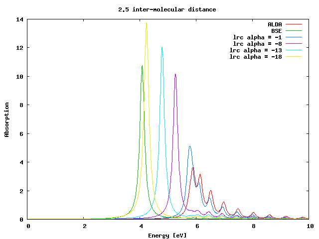
and run yambo. Now we can perform different calculations assigning different values to the variable LRC_alpha. This value is a static approximation to α(ω) in the long-range expression for fxc. This must be negative (the interaction between electron and hole is attractive). Try different numbers in the range 0 to -20. You will see that around LRC_alpha=-19 we obtain the same excitation energy of the BSE spectrum:
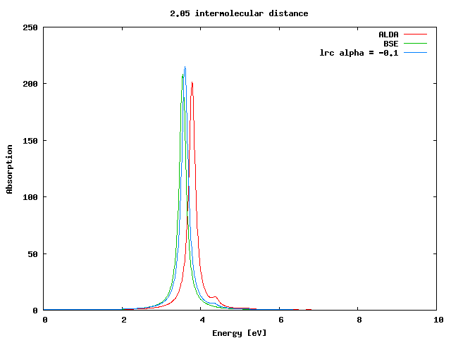
Now you can repeat the same calculations for the chain with 2.05 intermolecular distance. Once you will find the optimal value of %alpha, you will realize that as expected, it is one order of magnitude smaller than the one needed for the previous, more inhomogeneous system.
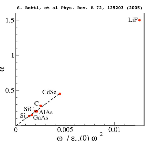
To conclude this tutorial note that the value of &alpha you found is much larger then in any solid, as showed in this picture. Can you understand why?
The Bethe-Salpeter Equation applied to 1D systems
The H2 hydrogen chain constitutes an example of a perfectly one-dimensional system. This property causes some tricky numerical problems that are, however, related to a precise physical process: the extreme confinement of 3D electrons in a small region of space. If we use yambo to perform a BS calculation you will immediately see where the problem is!
Let's move in the 2.5 folder
$ cd YAMBO_TUTORIALS/Hydrogen_Chain/YAMBO/2.5
We start by generating the input file. At the command line we have to tell yambo to construct the BSE (-o b) , to calculate the static screened interaction (-b), and to diagonalize the BS matrix (-y d), as well as activate a higher verbosity level in the input file -V qp:
$ yambo -o b -b -y d -V qp -F in_BSE
The generated input file describes our first attempt to calculate the excitonic polarization spectrum of the H chain. Let's now change the bolded values
BSEmod= "causal"             # [BSE] resonant/causal/coupling
BSENGBlk= 1   RL  # [BSK] Screened interaction block size
BSENGexx=  7659        RL    # [BSK] Exchange components
% BndsRnXs
1 | 20 |                     # [BSK] Bands range
%
NGsBlkXs= 1            RL    # [Xs] Response block size
First we consider only the resonant part of the BS equation:
BSEmod= "resonant"
Second, include a QP gap correction of 3.5 eV
% KfnQP_E
3.50000 | 1.000000 | 1.000000 |      # [EXTQP BSK BSS] E parameters (c/v)
%
Third, decide some reasonable size of the inverse dielectric function that defines the statically screened interaction (normally this has to be determined by convergence studies):
NGsBlkXs= 111
BSENGexx= 111
Fourth, you should change the BSE and polarization function band ranges:
% BSEBands
 1 | 2 |                   # [BSK] Bands range
%
% BndsRnXs
1 | 2 |          # [Xs] Polarization function bands
%
Two bands are enough in this case to get reasonable results.
Remember also to uncomment the variable WRbsWF if you want to plot the excitonic wave function afterwords.
Finally, we launch yambo
$ yambo -J BSE
and to our great surprise the polarization spectrum we obtain is completely wrong, with just a poor signal around 3eV which is nonsense:
As you can see the excitonic peak has even a negative intensity!
The reason of this serious failure of the BS calculation is due to the peculiar geometry of the H chain, and of corresponding BZ sampling that is strictly one dimensional. This is readily detected in any report file, like r_setup
 [...]
 [02.04] K-grid lattice
 ======================
 Compatible Grid is 1D
 B1 [rlu]= -0.01250   0.00000   0.00000
 Grid dimensions               :  80
 K lattice UC volume       [au]:   0.0011
As a consequence the region of space assigned to each k-point is strongly compressed in one of the dimensions, like the thin slices of this picture
The drastic consequence of this compression is that each region receives a piece of the electron-electron interaction that is multiplied by a form factor of the region, that, in general is assumed spatially constant. With such a severe sampling of the BZ this assumption is no longer valid and the screened interaction is anomalously enhanced.
To avoid this anomalous electron-electron interaction we use the Random Integration Method (-c option).
$ yambo -r -o b -b -y d -F in_BSE_RIM
and modify the RandQpts and RandGvec variables:
RandQpts= 1000000            # [RIM] Number of random q-points in the BZ
RandGvec= 1              RL  # [RIM] Coulomb interaction RS components
Here RandQpts specifies the number of random points to use and RandGvec the number of RL components to evaluate.
After launching
$ yambo -F in_BSE_RIM -J BSE_RIM
we notice a new section in the report file:
[04] Coulomb potential Random Integration (RIM)
=========
[RD./SAVE/ndb.RIM]------------------------------------------
 Brillouin Zone Q/K grids (IBZ/BZ):  41   80   41   80
 Coulombian RL components        : 1
 Coulombian diagonal components  :yes
 RIM random points               : 1000000
 RIM  RL volume             [a.u.]:  0.08864
 Real RL volume             [a.u.]:  0.08820
 Eps^-1 reference component       :0
 Eps^-1 components                :  0.00000   0.00000   0.00000
 RIM anisotropy factor            :  0.00000
- S/N 003292 ---------------------------------- v.02.09.09 -
Summary of Coulomb integrals for non-metallic bands |Q|[au] RIM/Bare:
 Q [1]:0.1000E-4  0.7653   * Q [2]:  0.01745  0.06494
 Q [3]:  0.03491  0.17408  * Q [4]:  0.05236  0.28906
 Q [5]:  0.06981  0.39545  * Q [6]:  0.08727  0.48820
 Q [7]: 0.104720  0.566608 * Q [8]: 0.122173 0.631844
 Q [9]: 0.139626  0.685750 * Q [10]: 0.157080 0.730229
 Q [11]: 0.174533 0.767000 * Q [12]: 0.191986 0.797519
 Q [13]: 0.209440 0.822983 * Q [14]: 0.226893 0.844352
 Q [15]: 0.244346 0.862396 * Q [16]: 0.261799 0.877727
 Q [17]: 0.279253 0.890832 * Q [18]: 0.296706 0.902101
 Q [19]: 0.314159 0.911847 * Q [20]: 0.331613 0.920320
 Q [21]: 0.349066 0.927727 * Q [22]: 0.366519 0.934233
 Q [23]: 0.383972 0.939973 * Q [24]: 0.401426 0.945061
 Q [25]: 0.418879 0.949588 * Q [26]: 0.436332 0.953633
 Q [27]: 0.453786 0.957260 * Q [28]: 0.471239 0.960523
 Q [29]: 0.488692 0.963470 * Q [30]: 0.506145 0.966138
 Q [31]: 0.523599 0.968561 * Q [32]: 0.541052 0.970768
 Q [33]: 0.558505 0.972783 * Q [34]: 0.575959 0.974629
 Q [35]: 0.593412 0.976322 * Q [36]: 0.610865 0.977879
 Q [37]: 0.628319 0.979314 * Q [38]: 0.645772 0.980640
 Q [39]: 0.663225 0.981867 * Q [40]: 0.680678 0.983004
 Q [41]: 0.698132 0.984061
The interesting result is that the 2nd and the 4th columns of numbers reflect the effect of the BZ compression: 1 means little effect, small numbers mean large effect. We see that the effect is huge for points in the BZ with small modulus (1st and 3rd columns).
The final BS polarizability is, now, physically correct and substantially different from ALDA:
Additional Exercises
The H chain is a one dimensional system, and, consequently it should not absorb when the light is polarized perpendicularly to the chain axis (the x direction).
- Repeat the RPA, ALDA, and BSE calculations for light polarized perpendicular to the chain axis to verify that the polarization is much smaller than in the parallel case.
- Use ypp to plot the excitonic wave function.
- Repeat the whole tutorial for the other interatomic distances.

