Silicon: Difference between revisions
(Created page with " === Basic concepts of the GW approximation === x300px|center| In this tutorial you will learn the basic concepts of the Hartree-Fock and of the GW...") |
|||
| (58 intermediate revisions by 7 users not shown) | |||
| Line 1: | Line 1: | ||
= Basic concepts of the GW approximation = | |||
[[File:GW0.png|x300px|center|]] | [[File:GW0.png|x300px|center|]] | ||
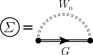
In this tutorial you will learn the basic concepts of the [[Hartree-Fock]] and of the | In this tutorial you will learn the basic concepts of the [[Hartree-Fock]] and of the GW<ref name="gw"/> approximation. In particular we will illustrate how to calculate [http://en.wikipedia.org/wiki/Quasiparticle Quasi-Particle] energies with a single shot G<sub>0</sub>W<sub>0</sub> approximation. Different lecture notes on the GW approach are available in the [[Lectures|Lectures section]]. | ||
The tutorial is split in different sections. In the first part we will deal with Hartree-Fock (HF) and the Coulomb-hole and screened-exchange (COHSEX) approximation. Finally in the last section we will discuss dynamical correlation with a Plasmon Pole Approximation (PPA). | The tutorial is split in different sections. In the first part we will deal with Hartree-Fock (HF) and the Coulomb-hole and screened-exchange (COHSEX) approximation. Finally in the last section we will discuss dynamical correlation with a Plasmon Pole Approximation (PPA). | ||
= The material: Silicon = | |||
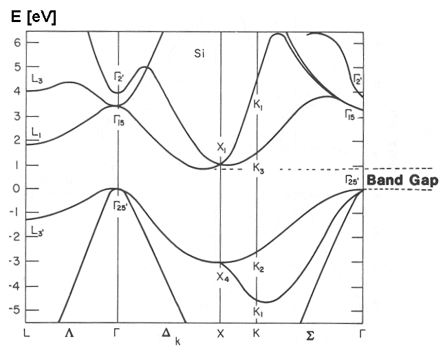
[[File:si_banddiagram.gif|thumb|x400px|Silicon Band Structure]] | |||
* [http://cst-www.nrl.navy.mil/lattice/struk/a1.html FCC] lattice | * [http://cst-www.nrl.navy.mil/lattice/struk/a1.html FCC] lattice | ||
| Line 14: | Line 15: | ||
* Lattice constant 10.183 [a.u.] | * Lattice constant 10.183 [a.u.] | ||
* Plane waves cutoff 15 Rydberg | * Plane waves cutoff 15 Rydberg | ||
* Direct gap 3.4 eV at Gamma | |||
* Indirect gap 1.1 eV between Gamma= (0 0 0) and a point X', | |||
[[ | = Tutorial files and Tutorial structure = | ||
Follow the instructions in [[Tutorials#Files]] and download/unpack the <code>Silicon.tar.gz</code>. | |||
Once the tutorial archive file is unzipped the following folder structure will appear | Once the tutorial archive file is unzipped the following folder structure will appear | ||
COPYING README | COPYING README Silicon/ | ||
with the Solid_Si folder containing | with the Solid_Si folder containing | ||
>ls | > ls Silicon/ | ||
Pwscf/ | PWSCF/ YAMBO/ | ||
In the Pwscf folder the student will find an input/output directory with input/output files for pw.x. The Silicon pseudopotential file is also provided. | |||
> ls PWSCF/ | |||
convergence_scripts input output psps | |||
In the | In the <code>convergence_scripts</code> you will find some useful shell scripts to run the ground state convergence runs for Silicon. | ||
The YAMBO folder contains the Yambo input/output files and core databases. | The YAMBO folder contains the Yambo input/output files and core databases. | ||
> ls YAMBO/ | |||
2x2x2/ 4x4x4/ 6x6x6/ 8x8x8/ Convergence_Plots_and_Scripts/ GAMMA/ | |||
The core databases are provided for several k-points grids. In addition the folder <code>Convergence_Plots_and_Scripts</code> contains some scripts to extract informations from the report files useful for the tutorial. | |||
= Hartree-Fock = | |||
Now we will study the convergence of the [http://en.wikipedia.org/wiki/Hartree%E2%80%93Fock_method Hartree-Fock] self energy, respect to the number of '''G'''-vectors and '''k'''-points. Yambo is a plane-wave code, therefore all the operators and wave-functions are expanded as: | Now we will study the convergence of the [http://en.wikipedia.org/wiki/Hartree%E2%80%93Fock_method Hartree-Fock] self energy, respect to the number of '''G'''-vectors and '''k'''-points. Yambo is a plane-wave code, therefore all the operators and wave-functions are expanded as: | ||
| Line 50: | Line 62: | ||
In order to generate the input file for the exchange type <code>yambo -x</code>. The variable that governs the number of '''G''' vectors N<sub>ex</sub> in the Coulomb potential is <code>EXXRLvcs</code>. In addition notice that in the previous formula for V('''r'''-'''r'''') we have an integral on the '''q''' vector, that in the code is discretized on a regular '''q'''-grid generated from the '''k'''-point one, '''q'''='''k'''-'''k''''. | In order to generate the input file for the exchange type <code>yambo -x</code>. The variable that governs the number of '''G''' vectors N<sub>ex</sub> in the Coulomb potential is <code>EXXRLvcs</code>. In addition notice that in the previous formula for V('''r'''-'''r'''') we have an integral on the '''q''' vector, that in the code is discretized on a regular '''q'''-grid generated from the '''k'''-point one, '''q'''='''k'''-'''k''''. | ||
== | == G-vectors convergence == | ||
Enter the <code>4x4x4</code> folder | |||
> cd 4x4x4 | |||
Now edit the <code>01HF_corrections</code> file changing the field <code>EXXRLvcs=</code>3,6,7 and 15 Ry. For each case run | |||
> yambo -F Inputs/01HF_corrections -J HF_XXRy | |||
<code>XX=</code>3,6,7 and 15 Ry | |||
Now plot the HF corrections by using the [[Gnuplot_scripts|hf_vs_cutoff.gnuplot]] script. Launch it via | |||
> | > gnuplot | ||
> | gnuplot>load "hf_vs_cutoff.gnuplot" | ||
Enter each grid folder and run | [[File:HF_parameters.png|Hartree-Fock corrections versus energy cutoff]] | ||
>yambo | |||
== K-points convergence== | |||
Enter each grid folder (<code>GAMMA,2x2x2,4x4x4,...</code>) and run | |||
> yambo | |||
without options. Then type | without options. Then type | ||
>yambo -x -F | > yambo -x -F Inputs/01HF_corrections -J 01HF_corrections | ||
and edit the 01HF_corrections file | and edit the 01HF_corrections file | ||
HF_and_locXC # [R XX] Hartree-Fock Self-energy and Vxc | HF_and_locXC # [R XX] Hartree-Fock Self-energy and Vxc | ||
EXXRLvcs= | EXXRLvcs= 15 Ry # [XX] Exchange RL components | ||
%QPkrange # [GW] QP generalized Kpoint/Band indices | %QPkrange # [GW] QP generalized Kpoint/Band indices | ||
1| 8| 1| 15| | 1| 8| 1| 15| | ||
| Line 77: | Line 102: | ||
setting | setting | ||
<code> EXXRLvcs= | <code> EXXRLvcs=15 Ry</code> | ||
Then run in each k-point folder | Then run in each k-point folder | ||
<code> | <code> > yambo -F Inputs/01HF_corrections -J 01HF_corrections</code> | ||
Note that after each run Yambo produces three output file, one starting with <code>r_...</code> , another with <code>l_...</code> and a third one starting with <code>o_...</code>. The first one is a ''report'' of the actual calculation with all the details of the system, input, and results, while the second is a ''log'' with the running time of each process. | |||
with <code> | The file we are most interested in is the output file, <code>o-01HF_corrections.hf</code>. This file contains several columns. The fourth, labelled with <code>Ehf</code> represents the Hartree-Fock energy. This is the quantity we have to look at. | ||
Use the [[Bash_scripts|parse_gap_hf.sh]] to parse the output files and adapt the gnuplot script provided earlier to print the values by using gnuplot. CAUTION: the provided bash script has been prepared for an old version of Yambo, most probably you need to update to the format of the Yambo version you are using. | |||
> cd ../ | |||
> ./parse_gap.sh o-01HF_corrections.hf hf_direct_gap_vs_kpoints.dat | |||
[[File:Hf gap vs kpts.png|Direct gap vs k-points]] | |||
= COHSEX without empty bands = | |||
The Hartree-Fock self-energy just described in the previous section, although successful on some molecular systems, miserably fails in extended systems. The reason of this failure lies in the fact that electrons can screen the Coulomb potential, and therefore one electron feels a screened potential instead of the bare one. A common approximation for this screened potential is the so-called Random Phase Approximation: | The Hartree-Fock self-energy just described in the previous section, although successful on some molecular systems, miserably fails in extended systems. The reason of this failure lies in the fact that electrons can screen the Coulomb potential, and therefore one electron feels a screened potential instead of the bare one. A common approximation for this screened potential is the so-called Random Phase Approximation: | ||
| Line 111: | Line 127: | ||
where the bare Coulomb potential V('''r''') is replaced by a non-local and frequency dependent one W('''r''','''r'''',ω). Subsequently it is possible to redefine all the perturbation theory in term of this screened potential, and disregarding the additional corrections coming from the vertex part, one obtains the so-called [[GW|GW]] approximation. | where the bare Coulomb potential V('''r''') is replaced by a non-local and frequency dependent one W('''r''','''r'''',ω). Subsequently it is possible to redefine all the perturbation theory in term of this screened potential, and disregarding the additional corrections coming from the vertex part, one obtains the so-called [[GW|GW]] approximation. | ||
However the substantial complexity associated with calculating the non-local, energy dependent Σ=GW operator inspired early efforts to find simplifying approximations as the static COHSEX approximation prosed by Hedin<ref | However the substantial complexity associated with calculating the non-local, energy dependent Σ=GW operator inspired early efforts to find simplifying approximations as the static COHSEX approximation prosed by Hedin<ref name="hedin"/>. The Coulomb Hole plus Screened Exchange (COHSEX) approximation[[[#march|2]],[[#fardi|3]]] eliminates the summation over empty states for the self energy operator and has the added benefit of being a static operator, a particular simplification for self consistent calculations. With the COHSEX approximation the self-energy is composed of two parts: | ||
[[File:gw_sex.png|Screened Exchange]] | [[File:gw_sex.png|Screened Exchange]] | ||
[[File:gw_coh.png|Cuolomb Hole]] | [[File:gw_coh.png|Cuolomb Hole]] | ||
where W<sub>p</sub>=W - V. | where W<sub>p</sub>=W - V. | ||
In order to calculate the COHSEX self-energy with yambo you need first the static screened interaction <code>yambo - | In order to calculate the COHSEX self-energy with yambo you need first the static screened interaction <code>yambo -X s -k hartree</code>. As for the V('''r''') case, also W('''r''','''r'''',E=0) will depend from the number of '''G'''-vectors, and the '''k'''-grid, but this time also the number of conduction bands <code>BndsRnXs</code> will enter in the screening calculation through the polarization function, see [http://www.yambo-code.org/theory/docs/doc_Xd.php The Interacting response function: Many-Body and TDDFT] section. Notice however that there are not any additional dependence of the self-energy operator from the conduction bands. After you obtained the screened interaction you are ready to build the self-energy operator and solve the corresponding Dyson equation, have a look to the [[GW|Dyson Equation solvers]] in Yambo. In order to get the quasi-particle energies, just do <code>yambo -X s -g n -k hartree</code>. After calculation are completed Yambo will produce an output file <code>o.qp</code> which contains the values of the bare and re-normalized energy levels. | ||
== K-points convergence == | |||
Follow the same strategy of the HF case. Enter each k-point folder and type | Follow the same strategy of the HF case. Enter each k-point folder and type | ||
>yambo - | > yambo -X s -k hartree -g n -p c -F Inputs/02Cohsex | ||
edit the input file and change the values of the fields | edit the input file and change the values of the fields | ||
EXXRLvcs=7 Ry %BndsRnXs 1 | 10 | # [Xs] Polarization function bands | EXXRLvcs=7 Ry | ||
%BndsRnXs | |||
1 | 10 | # [Xs] Polarization function bands | |||
% | |||
NGsBlkXs= 1 RL # [Xs] Response block size | NGsBlkXs= 1 RL # [Xs] Response block size | ||
#UseEbands # [GW] Force COHSEX to use empty bands | #UseEbands # [GW] Force COHSEX to use empty bands | ||
| Line 137: | Line 157: | ||
leaving the other parameters unchanged. Now, in each k-point folder, run | leaving the other parameters unchanged. Now, in each k-point folder, run | ||
>yambo -F | > yambo -F Inputs/02Cohsex -J Cohsex_HF7Ry_X0Ry-nb10 | ||
Adapt the shell script provided earlier to plot the direct gap dependence on the k-points grid. | |||
Please note at difference of the HF case, in the output is reported the COHSEX correction and not the COHSEX queasiparticle energy. | |||
[[File:Cohsex_HF7Ry_X0Ry-nb10_gap_vs_kpoints.png]] | |||
== W size convergence == | |||
Enter the <code>4x4x4</code> folder and edit the <code>02Cohsex_corrections</code> file changing the field <code>NGsBlkXs=</code>3,6,7 Ry. Run | Enter the <code>4x4x4</code> folder and edit the <code>02Cohsex_corrections</code> file changing the field <code>NGsBlkXs=</code>3,6,7 Ry. Run | ||
>yambo -F | > yambo -F Inputs/02Cohsex -J Cohsex_HF7Ry_X???Ry-nb10 | ||
with <code>???</code>=3,6,7 and 15 | with <code>???</code>=3,6,7 and 15. | ||
[[File:COHSEX_no_empties_W_size.png]] | |||
== W bands == | |||
%BndsRnXs | Open your input file and change only the input variable <code>NGsBlkXs=1 Ry</code>. Then change | ||
% BndsRnXs | |||
1 | 20 | # [Xs] Polarization function bands | |||
% | |||
and run <code>yambo -F Inputs/02Cohsex -J Cohsex_HF7Ry_X1Ry-nb20</code>. | |||
Repeat the calculations using 30 and 40 bands changing <code>nb???</code> in the job string identifier. Finally check how the Chosex Direct and Indirect band gap behave as a function of the number of bands in the screening. | |||
[[File:COHSEX_no_empties_W_bands.png]] | |||
== COHSEX with empty bands == | |||
While the Screened Exchange(SEX) part of the COHSEX self-energy has a structure similar to the Hartree-Fock exchange term, the Coulomb Hole(COH) acts as static external potential on the electrons. In the COH part the delta function δ('''r'''-'''r'''') comes from the completeness relation: | While the Screened Exchange(SEX) part of the COHSEX self-energy has a structure similar to the Hartree-Fock exchange term, the Coulomb Hole(COH) acts as static external potential on the electrons. In the COH part the delta function δ('''r'''-'''r'''') comes from the completeness relation: | ||
| Line 162: | Line 193: | ||
Now we avoid the use of this relation in such a way to have a self-energy that depends from the conduction bands too. This can be done uncommenting flags <code>UseEbands</code> and setting the number of bands in the Green's function: | Now we avoid the use of this relation in such a way to have a self-energy that depends from the conduction bands too. This can be done uncommenting flags <code>UseEbands</code> and setting the number of bands in the Green's function: | ||
UseEbands | |||
% GbndRnge | |||
1 | 10 | # [GW] G[W] bands range | |||
% | |||
Repeat the previous calculations with different <code>GbndRnge</code> for instance, 10 20 30 40, and check how the COHSEX direct and indirect band gap behave as a function of the number of bands in the Green's function. | |||
[[File:COHSEX_empties_G_bands.png]] | |||
[[File: | |||
= | = GW within the plasmon pole approximation (PPA) = | ||
Even the static COHSEX approximation is very appealing, it was clear from the first calculation that dynamical effects cannot be disregarded in solids | Even the static COHSEX approximation is very appealing, it was clear from the first calculation that dynamical effects cannot be disregarded in solids. This fact motivated the research for approximated way to deal with a frequency dependent interaction, and one of the first proposal was the so-called Plasmon-Pole Approximation (PPA). | ||
Now we will proceed to the calculation of the silicon band gap in G<sub>0</sub>W<sub>0</sub> within PPA. In each section you will be asked to perform several calculations varying the value of the relevant variables involved. More specifically let's consider a typical Yambo input file to calculate GW corrections in the PPA. | Now we will proceed to the calculation of the silicon band gap in G<sub>0</sub>W<sub>0</sub> within PPA. In each section you will be asked to perform several calculations varying the value of the relevant variables involved. More specifically let's consider a typical Yambo input file to calculate GW corrections in the PPA. | ||
| Line 185: | Line 217: | ||
% | % | ||
% BndsRnXp | % BndsRnXp | ||
1 | | 1 | 10 | # [Xp] Polarization function bands | ||
% | % | ||
NGsBlkXp= | NGsBlkXp= 1 RL # [Xp] Response block size | ||
% LongDrXp | % LongDrXp | ||
1.000000 | 0.000000 | 0.000000 | # [Xp] [cc] Electric Field | 1.000000 | 0.000000 | 0.000000 | # [Xp] [cc] Electric Field | ||
| Line 193: | Line 225: | ||
PPAPntXp= 27.21138 eV # [Xp] PPA imaginary energy | PPAPntXp= 27.21138 eV # [Xp] PPA imaginary energy | ||
% GbndRnge | % GbndRnge | ||
1 | | 1 | 10 | # [GW] G[W] bands range | ||
% | % | ||
GDamping= 0.10000 eV # [GW] G[W] damping | GDamping= 0.10000 eV # [GW] G[W] damping | ||
| Line 208: | Line 240: | ||
Follow the same strategy of the COHSEX case. Enter each k-point folder and type: | Follow the same strategy of the COHSEX case. Enter each k-point folder and type: | ||
>yambo -d -k hartree -g n -p p -F | > yambo -d -k hartree -g n -p p -F Inputs/03GoWo_PPA_corrections | ||
otherwise you can use the existent file <code>Input/03GoWo_PPA_corrections</code>. Now you have to study the convergence of the G<sub>0</sub>W<sub>0</sub> gap versus the number of k-points, the number of bands in χ <code>BndsRnXs</code>, the size of the dielectric constant <code>NGsBlkXs</code> and the number of bands in the Green's function <code>GbndRnge</code>. | otherwise you can use the existent file <code>Input/03GoWo_PPA_corrections</code>. Now you have to study the convergence of the G<sub>0</sub>W<sub>0</sub> gap versus the number of k-points, the number of bands in χ <code>BndsRnXs</code>, the size of the dielectric constant <code>NGsBlkXs</code> and the number of bands in the Green's function <code>GbndRnge</code>. | ||
| Line 214: | Line 246: | ||
Please follow the same strategy of the COHSEX case running yambo using | Please follow the same strategy of the COHSEX case running yambo using | ||
> yambo -F | > yambo -F Inputs/03GoWo_PPA_corrections -J GoWo_PPA_HF7Ry_X???Ry-nb???_nb???</code> | ||
The final convergence plots should look like these. | The final convergence plots should look like these (the plots are done using as a basis the above code). | ||
[[File:PPA W size.png]] | |||
[[File:PPA W bands.png]] | |||
[[File:PPA G bands.png]] | |||
[[File:PPA gap vs kpts.png]] | |||
Final runs!! Now you know how to converge a G<sub>0</sub>W<sub>0</sub> calculation so you can decide which are the parameters needed for full convergence. First do a COHSEX and then a GoWo (PPA) run at convergence, and you should obtain results similar to the following graph: | Final runs!! Now you know how to converge a G<sub>0</sub>W<sub>0</sub> calculation so you can decide which are the parameters needed for full convergence. First do a COHSEX and then a GoWo (PPA) run at convergence, and you should obtain results similar to the following graph: | ||
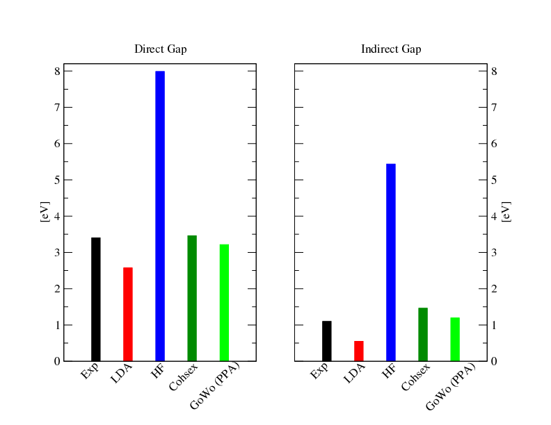
| Line 228: | Line 262: | ||
[[File:Si_gap.png|Final Gap Silicon]] | [[File:Si_gap.png|Final Gap Silicon]] | ||
= Advanced GW features = | |||
Some additional advanced GW features are possible with Yambo: | |||
* Taking into account the material anisotropy, see [https://www.yambo-code.eu/wiki/index.php/How_to_obtain_the_quasi-particle_band_structure_of_a_bulk_material:_h-BN#Step_7:_Taking_into_account_the_material_anisotropy Taking into account the material anisotropy] | |||
* Self consistency in G or GW in the eigenvalues, see [[Self-consistent GW on eigenvalues only]] | |||
= References = | |||
<references> | |||
<ref name="gw">H. N. Rojas, R. W. Godby, and R. J. Needs, Phys. Rev. Lett. '''74''', 1827 (1995)</ref> | |||
<ref name="hedin"> L. Hedin, Phys. Rev. '''139''', A796 (1965)</ref> | |||
</references> | |||
Latest revision as of 11:45, 17 January 2025
Basic concepts of the GW approximation
In this tutorial you will learn the basic concepts of the Hartree-Fock and of the GW[1] approximation. In particular we will illustrate how to calculate Quasi-Particle energies with a single shot G0W0 approximation. Different lecture notes on the GW approach are available in the Lectures section.
The tutorial is split in different sections. In the first part we will deal with Hartree-Fock (HF) and the Coulomb-hole and screened-exchange (COHSEX) approximation. Finally in the last section we will discuss dynamical correlation with a Plasmon Pole Approximation (PPA).
The material: Silicon
- FCC lattice
- Two atoms per cell (8 electrons)
- Lattice constant 10.183 [a.u.]
- Plane waves cutoff 15 Rydberg
- Direct gap 3.4 eV at Gamma
- Indirect gap 1.1 eV between Gamma= (0 0 0) and a point X',
Tutorial files and Tutorial structure
Follow the instructions in Tutorials#Files and download/unpack the Silicon.tar.gz.
Once the tutorial archive file is unzipped the following folder structure will appear
COPYING README Silicon/
with the Solid_Si folder containing
> ls Silicon/
PWSCF/  YAMBO/
In the Pwscf folder the student will find an input/output directory with input/output files for pw.x. The Silicon pseudopotential file is also provided.
> ls PWSCF/
convergence_scripts  input  output  psps
In the convergence_scripts you will find some useful shell scripts to run the ground state convergence runs for Silicon.
The YAMBO folder contains the Yambo input/output files and core databases.
> ls YAMBO/
2x2x2/  4x4x4/  6x6x6/  8x8x8/  Convergence_Plots_and_Scripts/  GAMMA/
The core databases are provided for several k-points grids. In addition the folder Convergence_Plots_and_Scripts contains some scripts to extract informations from the report files useful for the tutorial.
Hartree-Fock
Now we will study the convergence of the Hartree-Fock self energy, respect to the number of G-vectors and k-points. Yambo is a plane-wave code, therefore all the operators and wave-functions are expanded as:
Before you start any calculations we can decide how many G-vectors you want use to represent your wave-function. By default Yambo will use all of them, and for the present tutorial this is fine, however if you are studying larger systems you would like to reduce them in order to speed-up calculations, you can do it with yambo -i -V RL and then changing the variable MaxGvecs that referees to Ng in the previous formula.
Now we will proceed in the calculation of the Hartree-Fock exchange. This is composed of two terms, that Hartree and the Fock (or exchange) one:
In this tutorial we will calculate only the first order correction to the Kohn-Sham Hamiltonian due to the exchange term. Because of we are working in periodic system, the most appropriate basis to represent the Coulomb potential, appearing in the Fock term, is a plane-wave basis:
In order to generate the input file for the exchange type yambo -x. The variable that governs the number of G vectors Nex in the Coulomb potential is EXXRLvcs. In addition notice that in the previous formula for V(r-r') we have an integral on the q vector, that in the code is discretized on a regular q-grid generated from the k-point one, q=k-k'.
G-vectors convergence
Enter the 4x4x4 folder
> cd 4x4x4
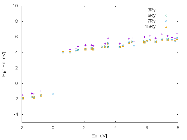
Now edit the 01HF_corrections file changing the field EXXRLvcs=3,6,7 and 15 Ry. For each case run
> yambo -F Inputs/01HF_corrections -J HF_XXRy
XX=3,6,7 and 15 Ry
Now plot the HF corrections by using the hf_vs_cutoff.gnuplot script. Launch it via
> gnuplot
gnuplot>load "hf_vs_cutoff.gnuplot"
K-points convergence
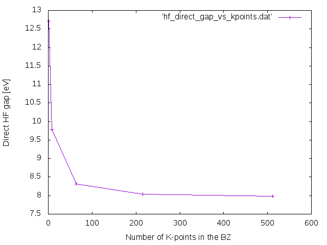
Enter each grid folder (GAMMA,2x2x2,4x4x4,...) and run
> yambo
without options. Then type
> yambo -x -F Inputs/01HF_corrections -J 01HF_corrections
and edit the 01HF_corrections file
HF_and_locXC                 # [R XX] Hartree-Fock Self-energy and Vxc
EXXRLvcs= 15           Ry    # [XX] Exchange RL components
%QPkrange                    # [GW] QP generalized Kpoint/Band indices
1|  8|  1| 15|
%
%QPerange                    # [GW] QP generalized Kpoint/Energy indices
 1|  8| 0.0|-1.0|
%
setting
EXXRLvcs=15 Ry
Then run in each k-point folder
> yambo -F Inputs/01HF_corrections -J 01HF_corrections
Note that after each run Yambo produces three output file, one starting with r_... , another with l_... and a third one starting with o_.... The first one is a report of the actual calculation with all the details of the system, input, and results, while the second is a log with the running time of each process.
The file we are most interested in is the output file, o-01HF_corrections.hf. This file contains several columns. The fourth, labelled with Ehf represents the Hartree-Fock energy. This is the quantity we have to look at.
Use the parse_gap_hf.sh to parse the output files and adapt the gnuplot script provided earlier to print the values by using gnuplot. CAUTION: the provided bash script has been prepared for an old version of Yambo, most probably you need to update to the format of the Yambo version you are using.
> cd ../
> ./parse_gap.sh o-01HF_corrections.hf hf_direct_gap_vs_kpoints.dat
COHSEX without empty bands
The Hartree-Fock self-energy just described in the previous section, although successful on some molecular systems, miserably fails in extended systems. The reason of this failure lies in the fact that electrons can screen the Coulomb potential, and therefore one electron feels a screened potential instead of the bare one. A common approximation for this screened potential is the so-called Random Phase Approximation:
where the bare Coulomb potential V(r) is replaced by a non-local and frequency dependent one W(r,r',ω). Subsequently it is possible to redefine all the perturbation theory in term of this screened potential, and disregarding the additional corrections coming from the vertex part, one obtains the so-called GW approximation.
However the substantial complexity associated with calculating the non-local, energy dependent Σ=GW operator inspired early efforts to find simplifying approximations as the static COHSEX approximation prosed by Hedin[2]. The Coulomb Hole plus Screened Exchange (COHSEX) approximation[[[#march|2]],3] eliminates the summation over empty states for the self energy operator and has the added benefit of being a static operator, a particular simplification for self consistent calculations. With the COHSEX approximation the self-energy is composed of two parts:
where Wp=W - V.
In order to calculate the COHSEX self-energy with yambo you need first the static screened interaction yambo -X s -k hartree. As for the V(r) case, also W(r,r',E=0) will depend from the number of G-vectors, and the k-grid, but this time also the number of conduction bands BndsRnXs will enter in the screening calculation through the polarization function, see The Interacting response function: Many-Body and TDDFT section. Notice however that there are not any additional dependence of the self-energy operator from the conduction bands. After you obtained the screened interaction you are ready to build the self-energy operator and solve the corresponding Dyson equation, have a look to the Dyson Equation solvers in Yambo. In order to get the quasi-particle energies, just do yambo -X s -g n -k hartree. After calculation are completed Yambo will produce an output file o.qp which contains the values of the bare and re-normalized energy levels.
K-points convergence
Follow the same strategy of the HF case. Enter each k-point folder and type
> yambo -X s -k hartree -g n -p c -F Inputs/02Cohsex
edit the input file and change the values of the fields
EXXRLvcs=7 Ry
%BndsRnXs
 1 | 10  |                   # [Xs] Polarization function bands
%
NGsBlkXs= 1            RL    # [Xs] Response block size
#UseEbands                   # [GW] Force COHSEX to use empty bands
%QPkrange                    # [GW] QP generalized Kpoint/Band indices
1|  8|  1| 10|
%
leaving the other parameters unchanged. Now, in each k-point folder, run
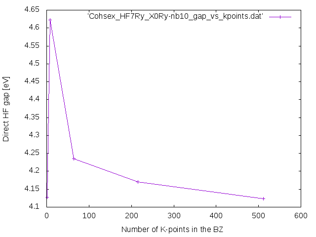
> yambo -F Inputs/02Cohsex -J Cohsex_HF7Ry_X0Ry-nb10
Adapt the shell script provided earlier to plot the direct gap dependence on the k-points grid. Please note at difference of the HF case, in the output is reported the COHSEX correction and not the COHSEX queasiparticle energy.
W size convergence
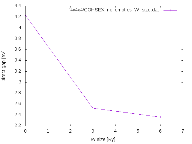
Enter the 4x4x4 folder and edit the 02Cohsex_corrections file changing the field NGsBlkXs=3,6,7 Ry. Run
> yambo -F Inputs/02Cohsex -J Cohsex_HF7Ry_X???Ry-nb10
with ???=3,6,7 and 15.
W bands
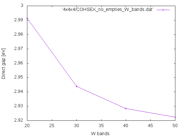
Open your input file and change only the input variable NGsBlkXs=1 Ry. Then change
% BndsRnXs
  1 | 20  |        # [Xs] Polarization function bands
%
and run yambo -F Inputs/02Cohsex -J Cohsex_HF7Ry_X1Ry-nb20.
Repeat the calculations using 30 and 40 bands changing nb??? in the job string identifier. Finally check how the Chosex Direct and Indirect band gap behave as a function of the number of bands in the screening.
COHSEX with empty bands
While the Screened Exchange(SEX) part of the COHSEX self-energy has a structure similar to the Hartree-Fock exchange term, the Coulomb Hole(COH) acts as static external potential on the electrons. In the COH part the delta function δ(r-r') comes from the completeness relation:
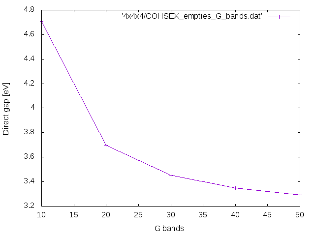
Now we avoid the use of this relation in such a way to have a self-energy that depends from the conduction bands too. This can be done uncommenting flags UseEbands and setting the number of bands in the Green's function:
UseEbands
% GbndRnge
  1 | 10 |                   # [GW] G[W] bands range
%
Repeat the previous calculations with different GbndRnge for instance, 10 20 30 40, and check how the COHSEX direct and indirect band gap behave as a function of the number of bands in the Green's function.
GW within the plasmon pole approximation (PPA)
Even the static COHSEX approximation is very appealing, it was clear from the first calculation that dynamical effects cannot be disregarded in solids. This fact motivated the research for approximated way to deal with a frequency dependent interaction, and one of the first proposal was the so-called Plasmon-Pole Approximation (PPA).
Now we will proceed to the calculation of the silicon band gap in G0W0 within PPA. In each section you will be asked to perform several calculations varying the value of the relevant variables involved. More specifically let's consider a typical Yambo input file to calculate GW corrections in the PPA.
gw0                          # [R GW] GoWo Quasiparticle energy levels
ppa                          # [R Xp] Plasmon Pole Approximation
HF_and_locXC                 # [R XX] Hartree-Fock Self-energy and Vxc
em1d                         # [R Xd] Dynamical Inverse Dielectric Matrix
EXXRLvcs= 7            Ry    # [XX] Exchange RL components
% QpntsRXp
  1 |  8 |                   # [Xp] Transferred momenta
%
% BndsRnXp
 1 | 10 |                 # [Xp] Polarization function bands
%
NGsBlkXp= 1            RL    # [Xp] Response block size
% LongDrXp
 1.000000 | 0.000000 | 0.000000 |        # [Xp] [cc] Electric Field
%
PPAPntXp= 27.21138     eV    # [Xp] PPA imaginary energy
% GbndRnge
 1 |  10 |                 # [GW] G[W] bands range
%
GDamping=  0.10000     eV    # [GW] G[W] damping
dScStep=  0.10000      eV    # [GW] Energy step to evalute Z factors
DysSolver= n               # [GW] Dyson Equation solver (`n`,`s`,`g`)
%QPkrange                    # [GW] QP generalized Kpoint/Band indices
 1|  8|  1| 10|
%
%QPerange                    # [GW] QP generalized Kpoint/Energy indices
 1|  8| 0.0|-1.0|
%
The variables are the same of the COHSEX case plus a new one PPAPntXp that describes the imaginary energy used to fit the Plasmon Pole model.
Follow the same strategy of the COHSEX case. Enter each k-point folder and type:
> yambo -d -k hartree -g n -p p -F Inputs/03GoWo_PPA_corrections
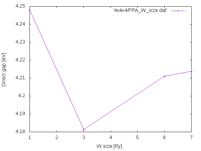
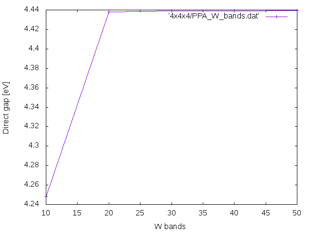
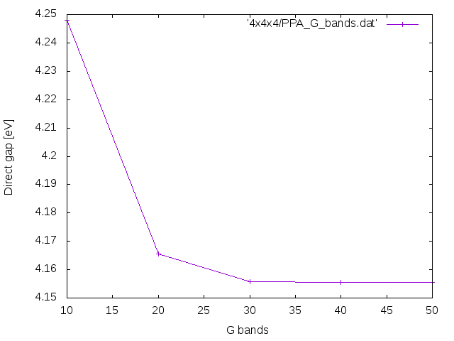
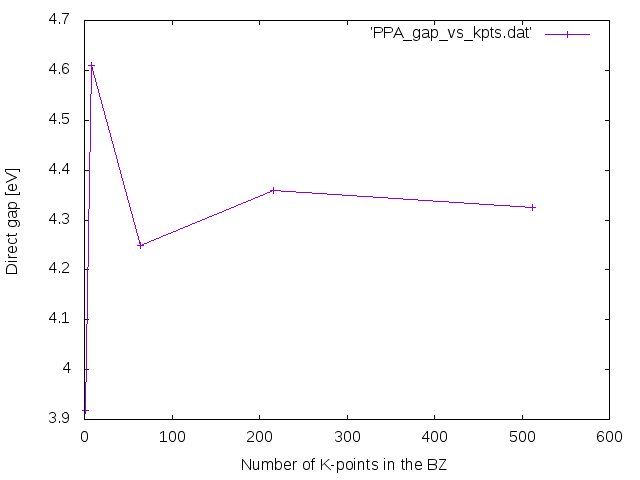
otherwise you can use the existent file Input/03GoWo_PPA_corrections. Now you have to study the convergence of the G0W0 gap versus the number of k-points, the number of bands in χ BndsRnXs, the size of the dielectric constant NGsBlkXs and the number of bands in the Green's function GbndRnge.
Please follow the same strategy of the COHSEX case running yambo using
> yambo -F Inputs/03GoWo_PPA_corrections -J GoWo_PPA_HF7Ry_X???Ry-nb???_nb???
The final convergence plots should look like these (the plots are done using as a basis the above code).
Final runs!! Now you know how to converge a G0W0 calculation so you can decide which are the parameters needed for full convergence. First do a COHSEX and then a GoWo (PPA) run at convergence, and you should obtain results similar to the following graph:
Advanced GW features
Some additional advanced GW features are possible with Yambo:
- Taking into account the material anisotropy, see Taking into account the material anisotropy
- Self consistency in G or GW in the eigenvalues, see Self-consistent GW on eigenvalues only
