How to choose the input parameters: Difference between revisions
(→Links) |
|||
| (24 intermediate revisions by 4 users not shown) | |||
| Line 1: | Line 1: | ||
In | In a [[Calculating optical spectra including excitonic effects: a step-by-step guide|previous tutorial]], you have been guided step-by-step through the calculations of the optical spectrum of bulk ''h-BN'' by solving the Bethe-Salpeter equation. The values for the relevant input parameters have then been given to you. | ||
In this tutorial you will learn how to choose these parameters which are related either to the truncation of infinite sums or to the approximations of infinitesimal with small, but finite quantities. A wrong choice of these parameters can lead to inaccurate or even physically wrong results. One needs to run a series of calculations by changing the parameters | In this tutorial you will learn how to choose these parameters which are related either to the truncation of infinite sums or to the approximations of infinitesimal with small, but finite quantities. A wrong choice of these parameters can lead to inaccurate or even physically wrong results. One needs to run a series of calculations by changing the parameters until the results are ''converged'', meaning they are changing by what you consider a negligible amount. This is a tedious yet essential part of determining the optical properties of a system. | ||
Note that all the operations described below can be automated. A flexible python-based interface to yambo, [ | Note that all the operations described below can be automated. A flexible python-based interface to yambo, [[First steps in Yambopy|yambopy]], can be used for this purpose. It is worth however to go at least once through the pain of a 'by-hand' convergence study so to better understand the automated process. | ||
==Before starting== | ==Before starting== | ||
Have completed (or be familiar with the content of) the following tutorials: | |||
* [[First steps: a walk through from DFT to optical properties]] | |||
* [[Calculating optical spectra including excitonic effects: a step-by-step guide]] | |||
==Background== | ==Background== | ||
| Line 40: | Line 36: | ||
Remember that the latter parameter appears only when the input is generated specifying the verbosity level <code>-V RL</code> | Remember that the latter parameter appears only when the input is generated specifying the verbosity level <code>-V RL</code> | ||
The convergence for the static screening then is similar to the convergence of other response functions and for the plasmon-pole in [[How to obtain the quasi-particle band structure of a bulk material: h-BN|GW calculations]] and won't be covered here. Note in fact that you can re-use the database obtained (and converged) from a previous | The convergence for the static screening then is similar to the convergence of other response functions and for the plasmon-pole in [[How to obtain the quasi-particle band structure of a bulk material: h-BN|GW calculations]] and won't be covered here. Note in fact that you can re-use the database obtained (and converged) from a previous screening calculation as long as the same k-points are used. | ||
==Convergence of the macroscopic dielectric function== | ==Convergence of the macroscopic dielectric function== | ||
| Line 65: | Line 61: | ||
===Prepare the common databases=== | ===Prepare the common databases=== | ||
Enter the <code> | |||
Enter the <code>hBN</code> directory (containing a 6x6x2 k-grid SAVE) and run the initialization if you didn't do it before. | |||
> cd YAMBO_TUTORIALS/hBN/YAMBO | |||
For all the calculations in this sessions you can fix the screening parameters, and thus calculate the screening once for all. | For all the calculations in this sessions you can fix the screening parameters, and thus calculate the screening once for all. | ||
Following the scheme we learned in previous tutorial: | Following the scheme we learned in previous tutorial: | ||
| Line 71: | Line 71: | ||
* Create the input for calculating the screening: | * Create the input for calculating the screening: | ||
> yambo -F 02_screening.in -X s | |||
* Modify the input as follows | * Modify the input as follows | ||
| Line 85: | Line 85: | ||
* Run the calculation for the screening | * Run the calculation for the screening | ||
> yambo -F 02_screening.in | |||
As we do not specify a particular prefix, the screening databases <code>ndb.dip_iR_and_P, ndb.em1s</code> are saved in the <code>SAVE</code> folder and visible to all the subsequent jobs you will launch is this directory. | As we do not specify a particular prefix, the screening databases <code>ndb.dip_iR_and_P, ndb.em1s</code> are saved in the <code>SAVE</code> folder and visible to all the subsequent jobs you will launch is this directory. | ||
| Line 91: | Line 91: | ||
===Convergence with the cut-off for reciprocal lattice vectors sums=== | ===Convergence with the cut-off for reciprocal lattice vectors sums=== | ||
As next step, create the input for calculating the macroscopic dielectric function: | As next step, create the input for calculating the macroscopic dielectric function: | ||
> yambo -F 03_bse.in -o b -k sex -y d -V qp | |||
Which combines the BS kernel + BS solver (diagonalization) runlevels | Which combines the BS kernel + BS solver (diagonalization) runlevels | ||
* Modify the input as follows | * Modify the input as follows | ||
| Line 113: | Line 113: | ||
% | % | ||
* Launch the calculation: | * Launch the calculation: | ||
> yambo -F 03_bse.in -J 3D_4Ry_GBlk | |||
This produces the file with the optical spectrum <code>o-3D_4Ry_GBlk.eps_q1_diago_bse</code>. | This produces the file with the optical spectrum <code>o-3D_4Ry_GBlk.eps_q1_diago_bse</code>. | ||
| Line 120: | Line 120: | ||
while leaving the rest untouched. | while leaving the rest untouched. | ||
* Launch the calculation: | * Launch the calculation: | ||
> yambo -F 03_bse.in -J 3D_3Ry_GBlk | |||
This produces the file with the optical spectrum <code>o-3D_3Ry_GBlk.eps_q1_diago_bse</code>. | This produces the file with the optical spectrum <code>o-3D_3Ry_GBlk.eps_q1_diago_bse</code>. | ||
* Repeat this operation for <code>BSENGBlk= '''2 Ry'''</code> and <code>BSENGBlk= '''1 Ry'''</code>. Remember to change the prefix correspondingly so that you can later on identify the job, e.g. <code>-J | * Repeat this operation for <code>BSENGBlk= '''2 Ry'''</code> and <code>BSENGBlk= '''1 Ry'''</code>. Remember to change the prefix correspondingly so that you can later on identify the job, e.g. <code>-J 3D_2Ry_GBlk</code> for <code>BSENGBlk='''2 Ry'''</code> etc. | ||
3D_2Ry_GBlk</code> for <code>BSENGBlk= '''2 Ry'''</code> | |||
* Finally plot the obtained optical spectra: | * Finally plot the obtained optical spectra: | ||
> gnuplot | |||
plot 'o-3D_4Ry_GBlk.eps_q1_diago_bse' w l t '4 Ry','o-3D_3Ry_GBlk.eps_q1_diago_bse' w l t '3 Ry', 'o-3D_2Ry_GBlk.eps_q1_diago_bse' w l t '2 Ry', 'o-3D_1Ry_GBlk.eps_q1_diago_bse' w l t '1 Ry' | plot 'o-3D_4Ry_GBlk.eps_q1_diago_bse' w l t '4 Ry','o-3D_3Ry_GBlk.eps_q1_diago_bse' w l t '3 Ry', 'o-3D_2Ry_GBlk.eps_q1_diago_bse' w l t '2 Ry', 'o-3D_1Ry_GBlk.eps_q1_diago_bse' w l t '1 Ry' | ||
| Line 134: | Line 133: | ||
This shows that <code>BSENGBlk= '''2 Ry'''</code> gives already a results close to convergence and we can confidently lower <code>BSENGBlk</code> to 2 or 3 Ry. | This shows that <code>BSENGBlk= '''2 Ry'''</code> gives already a results close to convergence and we can confidently lower <code>BSENGBlk</code> to 2 or 3 Ry. | ||
* Repeat now the same procedure with <code>BSENGexx</code>. Change the value to 10 Ry and 20 Ry. Remember to change the prefix correspondingly so that you can later on identify the job, e.g. <code>-J | * Repeat now the same procedure with <code>BSENGexx</code>. Change the value to 10 Ry and 20 Ry. Remember to change the prefix correspondingly so that you can later on identify the job, e.g. <code>-J 3D_10Ry_Gexx</code> for <code>BSENGexx= '''10 Ry'''</code> etc., and remember to keep the value of <code>BSENGBlk</code> the same throughout these calculations. | ||
3D_10Ry_Gexx</code> for <code>BSENGexx= '''10 Ry'''</code>. | |||
* Finally plot the obtained optical spectra: | * Finally plot the obtained optical spectra: | ||
> gnuplot | |||
plot 'o-3D_4Ry_GBlk.eps_q1_diago_bse' w l t '30 Ry' ls 1,'o-3D_20Ry_Gexx.eps_q1_diago_bse' w l t '20 Ry', 'o-3D_10Ry_Gexx.eps_q1_diago_bse' w l t '10 Ry' | plot 'o-3D_4Ry_GBlk.eps_q1_diago_bse' w l t '30 Ry' ls 1,'o-3D_20Ry_Gexx.eps_q1_diago_bse' w l t '20 Ry', 'o-3D_10Ry_Gexx.eps_q1_diago_bse' w l t '10 Ry' | ||
| Line 158: | Line 156: | ||
* Plot the optical spectra obtained from the different runs: | * Plot the optical spectra obtained from the different runs: | ||
> gnuplot | |||
plot 'o-3D_4Ry_GBlk.eps_q1_diago_bse' w l t '6-10 Bands','o-3D_7-10_BND.eps_q1_diago_bse' w l t '7-10 Bands', 'o-3D_8-10_BND.eps_q1_diago_bse' w l t '8-10 Bands' | plot 'o-3D_4Ry_GBlk.eps_q1_diago_bse' w l t '6-10 Bands','o-3D_7-10_BND.eps_q1_diago_bse' w l t '7-10 Bands', 'o-3D_8-10_BND.eps_q1_diago_bse' w l t '8-10 Bands' | ||
plot 'o-3D_4Ry_GBlk.eps_q1_diago_bse' w l t '6-10 Bands','o-3D_6-9_BND.eps_q1_diago_bse' w l t '6-9 Bands', 'o-3D_7-9_BND.eps_q1_diago_bse' w l t '7-9 Bands', 'o-3D_8-9_BND.eps_q1_diago_bse' w l t '8-9 Bands' | plot 'o-3D_4Ry_GBlk.eps_q1_diago_bse' w l t '6-10 Bands','o-3D_6-9_BND.eps_q1_diago_bse' w l t '6-9 Bands', 'o-3D_7-9_BND.eps_q1_diago_bse' w l t '7-9 Bands', 'o-3D_8-9_BND.eps_q1_diago_bse' w l t '8-9 Bands' | ||
[[File:03 | [[File:03 band convergence 1.png|500px|left|Band convergence]] [[File:03 band convergence2.png|500px|center|Band convergence 2]] | ||
The plots show that we need to include valence bands from at least 6-7 (those bands are degenerate at several high symmetry points of the Brillouin zone) and conduction at least up to band 10. | The plots show that we need to include valence bands from at least 6-7 (those bands are degenerate at several high symmetry points of the Brillouin zone) and conduction at least up to band 10. | ||
| Line 168: | Line 166: | ||
For example you can prepare and run calculations with the following bands ranges: ''1-12'', ''4-12'', ''4-14'' and plot the results: | For example you can prepare and run calculations with the following bands ranges: ''1-12'', ''4-12'', ''4-14'' and plot the results: | ||
> gnuplot | |||
plot 'o-3D_4Ry_GBlk.eps_q1_diago_bse' w l t '6-10 Bands','o-3D_4-12_BND.eps_q1_diago_bse' w l t '4-12 Bands', 'o-3D_4-14_BND.eps_q1_diago_bse' w l t '4-14 Bands', 'o-3D_1-12_BND.eps_q1_diago_bse' w l t '1-12 Bands' ls 4 | plot 'o-3D_4Ry_GBlk.eps_q1_diago_bse' w l t '6-10 Bands','o-3D_4-12_BND.eps_q1_diago_bse' w l t '4-12 Bands', 'o-3D_4-14_BND.eps_q1_diago_bse' w l t '4-14 Bands', 'o-3D_1-12_BND.eps_q1_diago_bse' w l t '1-12 Bands' ls 4 | ||
| Line 178: | Line 176: | ||
As final step you need to study the dependence on the '''k''' mesh. This parameter cannot be changed in yambo. For each '''k''' mesh you need to run a separate non-self consistent DFT calculation (on top of a converged self-consistent one) and generate the corresponding SAVE folders. Be careful to change '''only''' the '''k''' mesh. | As final step you need to study the dependence on the '''k''' mesh. This parameter cannot be changed in yambo. For each '''k''' mesh you need to run a separate non-self consistent DFT calculation (on top of a converged self-consistent one) and generate the corresponding SAVE folders. Be careful to change '''only''' the '''k''' mesh. | ||
For this exercise the SAVE databases for different meshes were generated beforehand and are contained in the corresponding folders: | For this exercise the SAVE databases for different meshes were generated beforehand in the [http://www.yambo-code.org/educational/tutorials/files/hBN-convergence-kpoints.tar.gz hBN-convergence-kpoints.tar.gz] tarball and are contained in the corresponding folders: | ||
> pwd | |||
YAMBO_TUTORIALS/hBN-convergence-kpoints/YAMBO | |||
> ls | |||
9x9x3 12x12x4 15x15x5 18x18x6 | 9x9x3 12x12x4 15x15x5 18x18x6 | ||
| Line 186: | Line 187: | ||
* Run the initialization | * Run the initialization | ||
* Create the input for calculating the screening: | * Create the input for calculating the screening: | ||
> yambo -F 02_screening.in -J 3D_993 -X s | |||
* Modify the input as follows | * Modify the input as follows | ||
[[Variables#NGsBlkXs|NGsBlkXs]] = 4 Ry | [[Variables#NGsBlkXs|NGsBlkXs]] = 4 Ry | ||
| Line 196: | Line 197: | ||
% | % | ||
* Run the calculation for the screening | * Run the calculation for the screening | ||
> yambo -F 02_screening.in -J 3D_993 | |||
* Create the input for calculating the macroscopic dielectric function: | * Create the input for calculating the macroscopic dielectric function: | ||
> yambo -F 03_bse.in -J 3D_993 -o b -k sex -y h -V qp | |||
Which combines the BS kernel + BS solver (Lanczos-Haydock) runlevels | Which combines the BS kernel + BS solver (Lanczos-Haydock) runlevels | ||
* Modify the input as follows | * Modify the input as follows | ||
| Line 221: | Line 222: | ||
[[Variables#BSHayTrs|BSHayTrs]]= 0.02000 | [[Variables#BSHayTrs|BSHayTrs]]= 0.02000 | ||
* Launch the calculation: | * Launch the calculation: | ||
> yambo -F 03_bse.in -J 3D_993 | |||
* Repeat the procedure for the <code>12x12x4</code> (it will take few minutes) with the difference you will use a different prefix: <code>-J 3D_12124</code>. | * Repeat the procedure for the <code>12x12x4</code> (it will take few minutes) with the difference you will use a different prefix: <code>-J 3D_12124</code>. | ||
| Line 228: | Line 229: | ||
Note that for those meshes the BS kernel database is becoming very/too large and you need to fragment it. To do that '''after''' you generated and modified the input invoke yambo again as: | Note that for those meshes the BS kernel database is becoming very/too large and you need to fragment it. To do that '''after''' you generated and modified the input invoke yambo again as: | ||
> yambo -F 03_bse.in -J 3D_15155 -o b -k sex -y h '''-V io''' | |||
and modify the variable | and modify the variable | ||
[[Variables#DBsFRAGpm|DBsFRAGpm]]= "+BS" | [[Variables#DBsFRAGpm|DBsFRAGpm]]= "+BS" | ||
Then launch the calculation | Then launch the calculation | ||
> yambo -F 03_bse.in -J 3D_15155 | |||
If you correctly followed the above procedure you should have a file with the optical absorption spectrum for each mesh, e.g. <code>o-3D_993.eps_q1_haydock_bse</code>. | If you correctly followed the above procedure you should have a file with the optical absorption spectrum for each mesh, e.g. <code>o-3D_993.eps_q1_haydock_bse</code>. | ||
To see the effect of k-points plot those files with <code>gnuplot</code>: | To see the effect of k-points plot those files with <code>gnuplot</code> (remember to include the 6x6x2 calculation which should still be inside <code>hBN/YAMBO</code>, if the parameters don't match you simply rerun it here by creating a <code>6x6x2</code> directory and copying the SAVE there): | ||
> gnuplot | |||
plot '18x18x6/o-3D_18186.eps_q1_haydock_bse' w l t '18x18x6, '15x15x5/o-3D_15155.eps_q1_haydock_bse' w l t '15x15x5','12x12x4/o-3D_12124.eps_q1_haydock_bse' w l t '12x12x4, | plot '18x18x6/o-3D_18186.eps_q1_haydock_bse' w l t '18x18x6, '15x15x5/o-3D_15155.eps_q1_haydock_bse' w l t '15x15x5','12x12x4/o-3D_12124.eps_q1_haydock_bse' w l t '12x12x4, | ||
'9x9x3/o-3D_993.eps_q1_haydock_bse' w l t '9x9x3', '6x6x2/o-3D_662.eps_q1_haydock_bse' w l t '6x6x2' | '9x9x3/o-3D_993.eps_q1_haydock_bse' w l t '9x9x3', '6x6x2/o-3D_662.eps_q1_haydock_bse' w l t '6x6x2' | ||
| Line 256: | Line 257: | ||
* <code>BSEBands '''from 6 to 10'''</code> | * <code>BSEBands '''from 6 to 10'''</code> | ||
* To converge the position and shape of the first exciton peak a 12x12x4 mesh is sufficient. For the second exciton peak a mesh larger than 18x18x6 would be needed (indeed Wirtz and co-workers found a k-mesh 24x24x10 was needed.<ref>Ludger Wirtz, Andrea Marini, Myrta Gruning, Angel Rubio in arXiv:cond-mat/0508421 [cond-mat.mtrl-sci]</ref>) | * To converge the position and shape of the first exciton peak a 12x12x4 mesh is sufficient. For the second exciton peak a mesh larger than 18x18x6 would be needed (indeed Wirtz and co-workers found a k-mesh 24x24x10 was needed.<ref>Ludger Wirtz, Andrea Marini, Myrta Gruning, Angel Rubio in arXiv:cond-mat/0508421 [cond-mat.mtrl-sci]</ref>) | ||
==Links== | |||
* Go to [[Calculating optical spectra including excitonic effects: a step-by-step guide]] module | |||
* Back to [[Modena 2025]] | |||
* Back to [[Rome 2023#Tutorials]] | |||
* Back to [[BSE hBN Yambo Virtual 2021 version|BSE tutorial sections]] | |||
* Back to [[ICTP 2022]] | |||
* Back to [[CECAM VIRTUAL 2021]] | |||
* [[Modules|Back to technical modules menu]] | |||
* [[Tutorials|Back to tutorials menu]] | |||
==References== | ==References== | ||
Latest revision as of 14:13, 21 May 2025
In a previous tutorial, you have been guided step-by-step through the calculations of the optical spectrum of bulk h-BN by solving the Bethe-Salpeter equation. The values for the relevant input parameters have then been given to you.
In this tutorial you will learn how to choose these parameters which are related either to the truncation of infinite sums or to the approximations of infinitesimal with small, but finite quantities. A wrong choice of these parameters can lead to inaccurate or even physically wrong results. One needs to run a series of calculations by changing the parameters until the results are converged, meaning they are changing by what you consider a negligible amount. This is a tedious yet essential part of determining the optical properties of a system.
Note that all the operations described below can be automated. A flexible python-based interface to yambo, yambopy, can be used for this purpose. It is worth however to go at least once through the pain of a 'by-hand' convergence study so to better understand the automated process.
Before starting
Have completed (or be familiar with the content of) the following tutorials:
- First steps: a walk through from DFT to optical properties
- Calculating optical spectra including excitonic effects: a step-by-step guide
Background
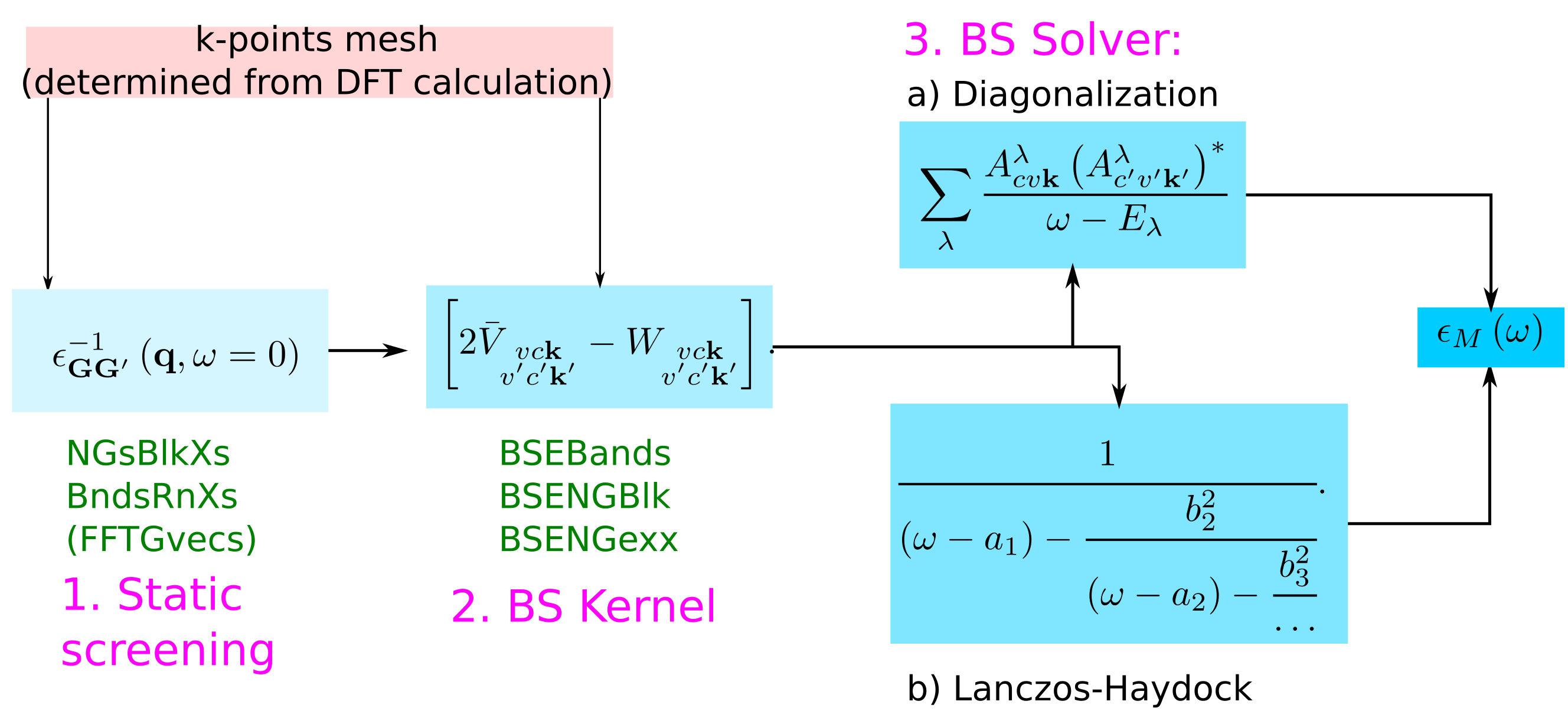
Coming back to the scheme to calculate the macroscopic dielectric matrix within Bethe-Salpeter (BS), the list of the parameters that have to be determined by convergence studies are:
This provides as well a scheme for a full convergence study:
- first the parameters for the screening have to be determined,
- then the parameters for the BS kernel, and
- finally the convergence with respect to the choice of the k-mesh needs to performed.
Convergence of the static screening
The parameters that need to be converged can be understood by looking at the equations:
where χGG' is given by
NGsBlkXs: The dimension of the microscopic inverse matrix, related to Local fieldsBndsRnXs: The sum on bands in the independent particle χ0GG'
Furthermore as shown in this tutorial one can reduce the value of
since generally, fewer G-vectors are needed than what are needed in DFT calculations. This can be critical for large calculations, or for supercells with a lot of vacuum.
Remember that the latter parameter appears only when the input is generated specifying the verbosity level -V RL
The convergence for the static screening then is similar to the convergence of other response functions and for the plasmon-pole in GW calculations and won't be covered here. Note in fact that you can re-use the database obtained (and converged) from a previous screening calculation as long as the same k-points are used.
Convergence of the macroscopic dielectric function
In the expression for the macroscopic dielectric function
depends on the summation over the pair of quasiparticle states vck.
BSEBands: defines the vc pairs.- the k-point mesh of the DFT calculations defines the k
Basically we need a large enough basis of transitions (pair of quasiparticle states) to correctly describe the excitons (in the energy region of interest).
Furthermore, in the kernel components
the summations over G vectors appear. These corresponds to two parameters:
BSENGblk: defines the screened interaction block size (double sum in W), related to the electron-hole attraction.BSENGexx: defines the components of Hartree potential (the sum in V), related to local fields.
In the following we will see how the spectrum depends on these parameters.
Prepare the common databases
Enter the hBN directory (containing a 6x6x2 k-grid SAVE) and run the initialization if you didn't do it before.
> cd YAMBO_TUTORIALS/hBN/YAMBO
For all the calculations in this sessions you can fix the screening parameters, and thus calculate the screening once for all. Following the scheme we learned in previous tutorial:
- Create the input for calculating the screening:
> yambo -F 02_screening.in -X s
- Modify the input as follows
NGsBlkXs = 4 Ry
%BndsRnXs
 1 | 40 |
%
%LongDrXS
 1.000 | 1.000 | 1.000|
%
- Run the calculation for the screening
> yambo -F 02_screening.in
As we do not specify a particular prefix, the screening databases ndb.dip_iR_and_P, ndb.em1s are saved in the SAVE folder and visible to all the subsequent jobs you will launch is this directory.
Convergence with the cut-off for reciprocal lattice vectors sums
As next step, create the input for calculating the macroscopic dielectric function:
> yambo -F 03_bse.in -o b -k sex -y d -V qp
Which combines the BS kernel + BS solver (diagonalization) runlevels
- Modify the input as follows
BSENGexx = 30 Ry
BSENGBlk = 4 Ry
% BSEBands
 6 | 10 |
%
% BEnRange
  2.00000 | 8.00000 | eV
%
BEnSteps= 100
% BDmRange
  0.10000 |  0.10000 | eV
%
% BLongDir
 1.000000 | 1.000000 | 0.000000 |
%
% KfnQP_E
 1.440000 | 1.000000 | 1.000000 |
%
- Launch the calculation:
> yambo -F 03_bse.in -J 3D_4Ry_GBlk
This produces the file with the optical spectrum o-3D_4Ry_GBlk.eps_q1_diago_bse.
- Open the
03_bse.inin an editor and changes:
BSENGBlk = 3 Ry
while leaving the rest untouched.
- Launch the calculation:
> yambo -F 03_bse.in -J 3D_3Ry_GBlk
This produces the file with the optical spectrum o-3D_3Ry_GBlk.eps_q1_diago_bse.
- Repeat this operation for
BSENGBlk= 2 RyandBSENGBlk= 1 Ry. Remember to change the prefix correspondingly so that you can later on identify the job, e.g.-J 3D_2Ry_GBlkforBSENGBlk=2 Ryetc.
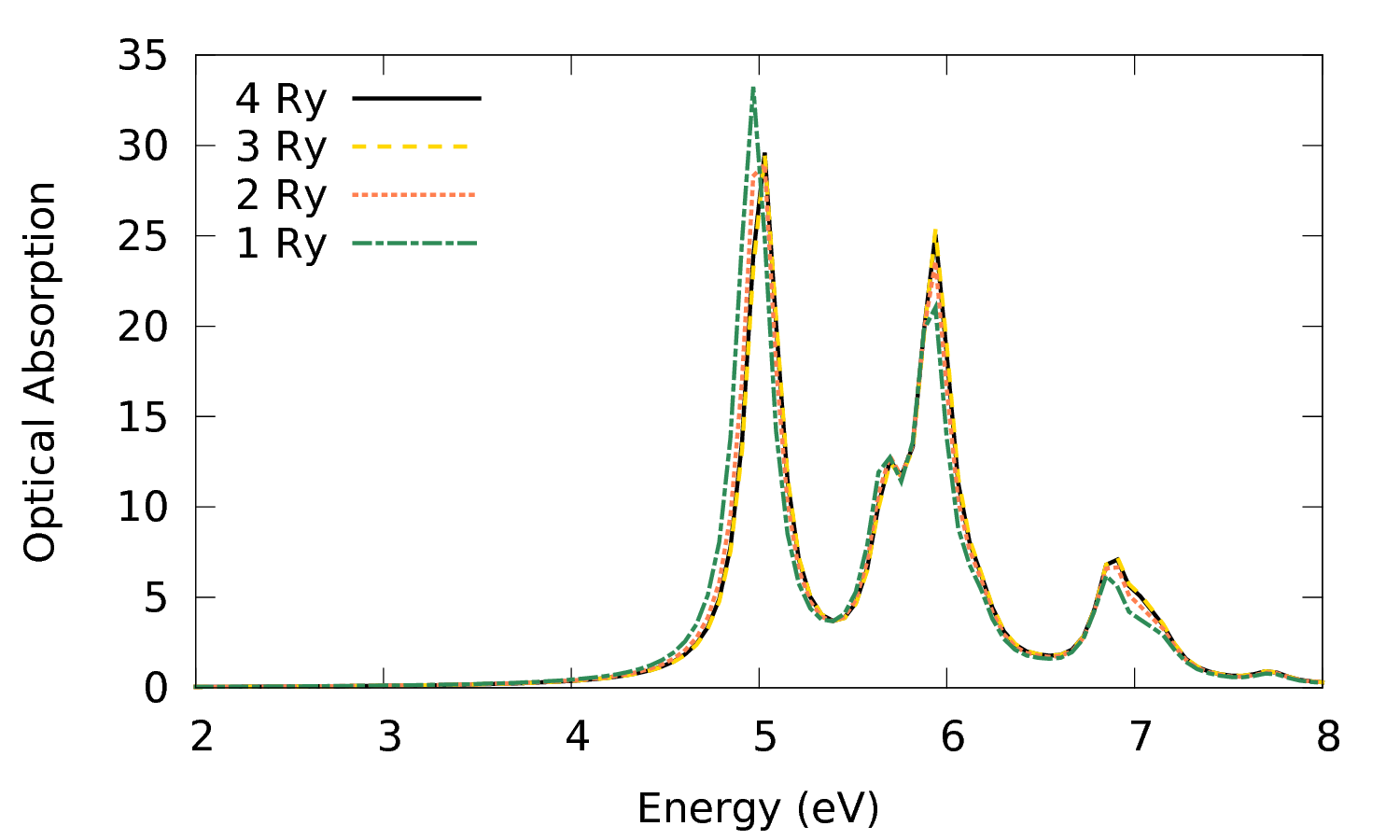
- Finally plot the obtained optical spectra:
> gnuplot
plot  'o-3D_4Ry_GBlk.eps_q1_diago_bse' w l t '4 Ry','o-3D_3Ry_GBlk.eps_q1_diago_bse' w l t '3 Ry',  'o-3D_2Ry_GBlk.eps_q1_diago_bse' w l t '2 Ry', 'o-3D_1Ry_GBlk.eps_q1_diago_bse' w l t '1 Ry'
This shows that BSENGBlk= 2 Ry gives already a results close to convergence and we can confidently lower BSENGBlk to 2 or 3 Ry.
- Repeat now the same procedure with
BSENGexx. Change the value to 10 Ry and 20 Ry. Remember to change the prefix correspondingly so that you can later on identify the job, e.g.-J 3D_10Ry_GexxforBSENGexx= 10 Ryetc., and remember to keep the value ofBSENGBlkthe same throughout these calculations.
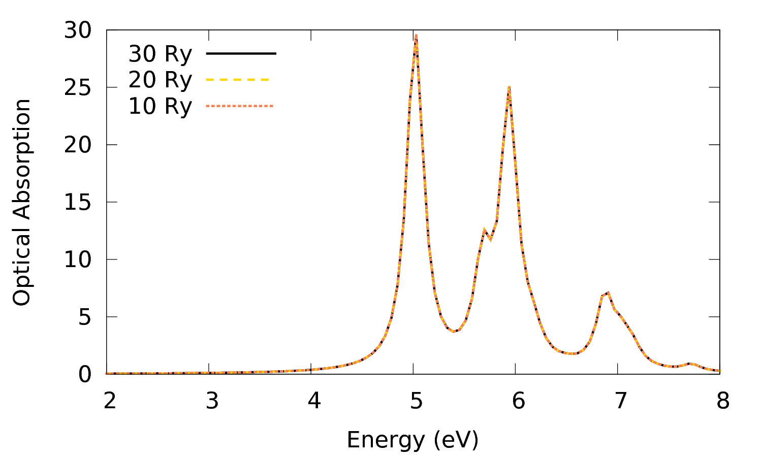
- Finally plot the obtained optical spectra:
> gnuplot
 plot  'o-3D_4Ry_GBlk.eps_q1_diago_bse' w l t '30 Ry' ls 1,'o-3D_20Ry_Gexx.eps_q1_diago_bse' w l t '20 Ry',  'o-3D_10Ry_Gexx.eps_q1_diago_bse' w l t '10 Ry'
The plot shows that already with BSENGexx= 10 Ry the spectrum is converged and the cut-off can be lowered to this value.
Convergence with the BS bands
You can now repeat the procedure above keeping fixed all parameters to their original values except for
% BSEBands
6 | 10 |
%
Typically only the bands which are close to the Fermi energies contributes to the spectrum. If the energy separation between two bands is much larger than the spectral energy range, you can assume the corresponding transitions are not contributing to the spectra.
- Repeat then the calculation for the optical spectrum using the following band ranges:
7-10, 8-10, 6-9, 7-9 and 8-9.
When launching the job remember to identify your job with a recognizable name, e.g. -J 3D_7-9_BND for the 7-9 range.
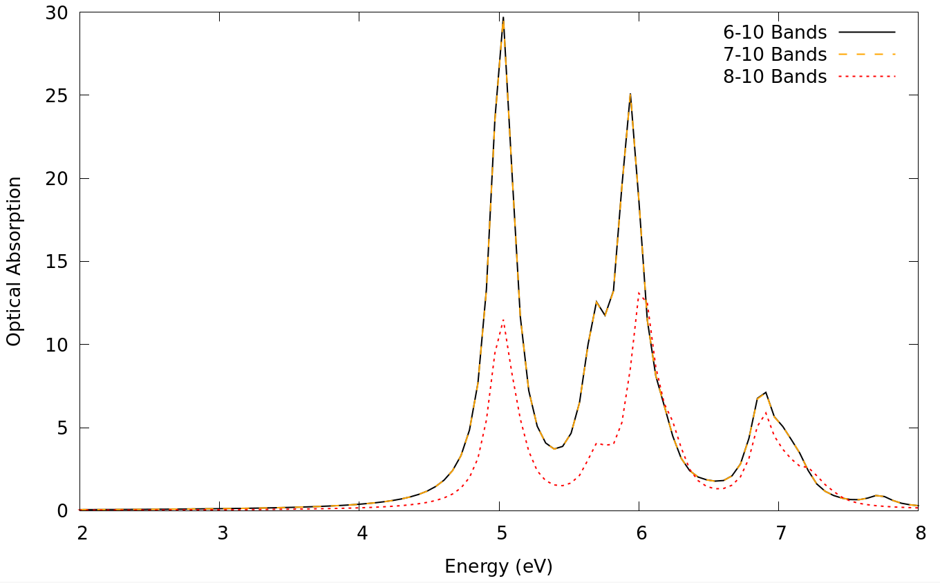
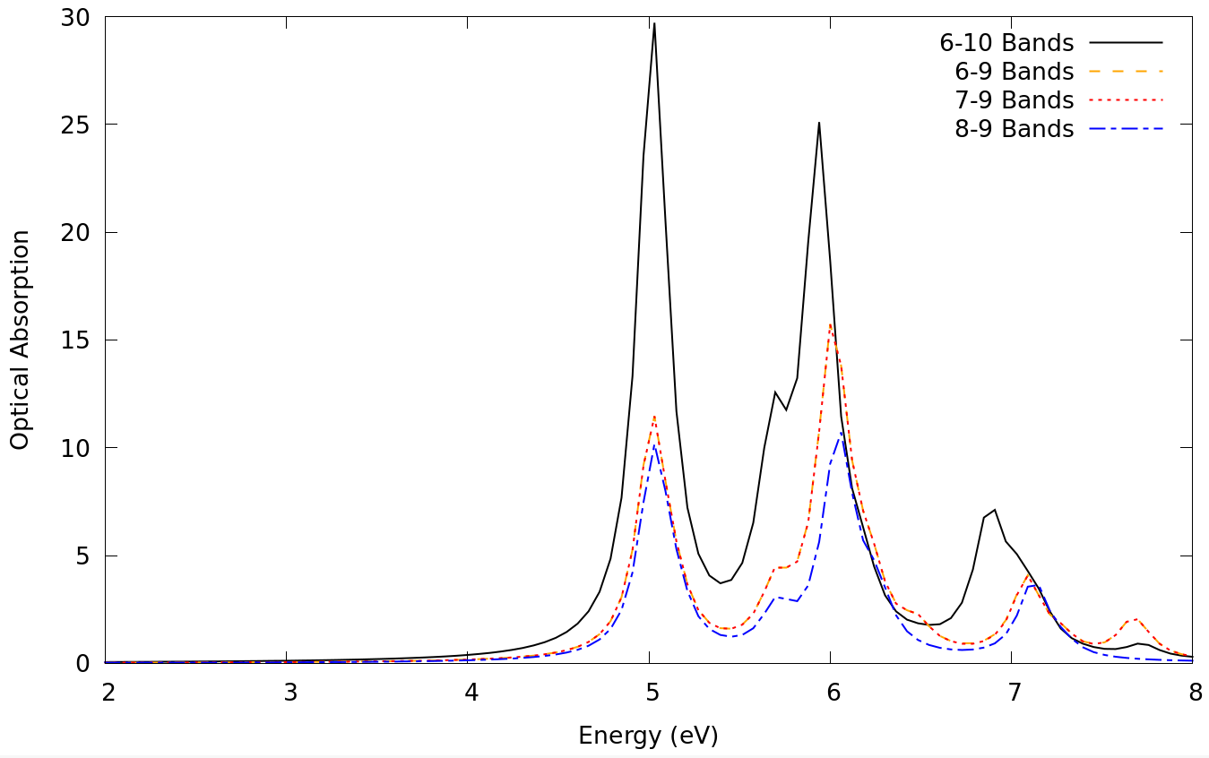
- Plot the optical spectra obtained from the different runs:
> gnuplot
plot  'o-3D_4Ry_GBlk.eps_q1_diago_bse' w l t '6-10 Bands','o-3D_7-10_BND.eps_q1_diago_bse' w l t '7-10 Bands', 'o-3D_8-10_BND.eps_q1_diago_bse' w l t '8-10 Bands'
plot  'o-3D_4Ry_GBlk.eps_q1_diago_bse' w l t '6-10 Bands','o-3D_6-9_BND.eps_q1_diago_bse' w l t '6-9 Bands', 'o-3D_7-9_BND.eps_q1_diago_bse' w l t '7-9 Bands', 'o-3D_8-9_BND.eps_q1_diago_bse' w l t '8-9 Bands'
The plots show that we need to include valence bands from at least 6-7 (those bands are degenerate at several high symmetry points of the Brillouin zone) and conduction at least up to band 10. To see if this is sufficient you can try to include more bands.
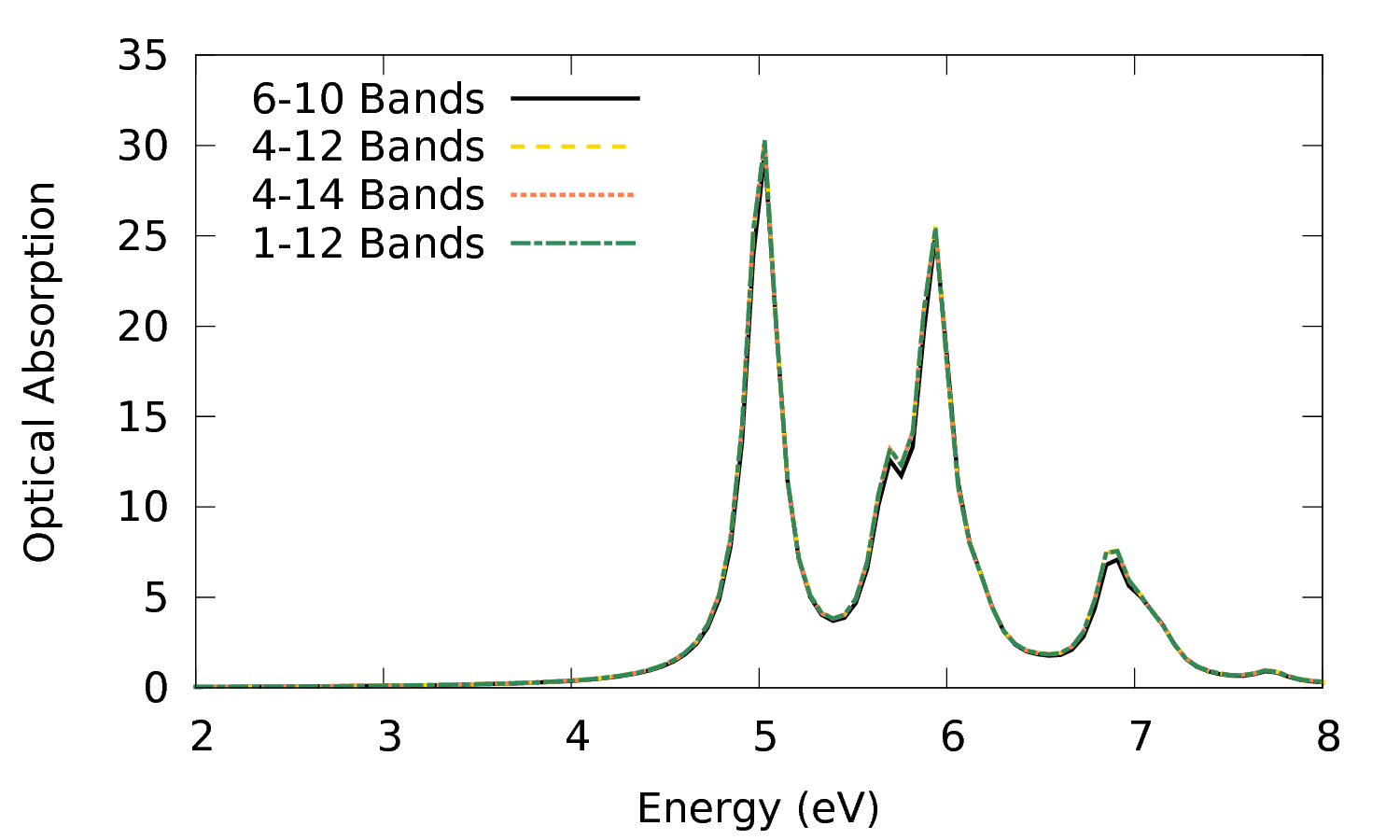
For example you can prepare and run calculations with the following bands ranges: 1-12, 4-12, 4-14 and plot the results:
> gnuplot
plot  'o-3D_4Ry_GBlk.eps_q1_diago_bse' w l t '6-10 Bands','o-3D_4-12_BND.eps_q1_diago_bse' w l t '4-12 Bands', 'o-3D_4-14_BND.eps_q1_diago_bse' w l t '4-14 Bands', 'o-3D_1-12_BND.eps_q1_diago_bse' w l t '1-12 Bands' ls 4
The plot is showing that the spectrum changes only marginally when adding those bands.
Convergence with the k-point mesh
As final step you need to study the dependence on the k mesh. This parameter cannot be changed in yambo. For each k mesh you need to run a separate non-self consistent DFT calculation (on top of a converged self-consistent one) and generate the corresponding SAVE folders. Be careful to change only the k mesh.
For this exercise the SAVE databases for different meshes were generated beforehand in the hBN-convergence-kpoints.tar.gz tarball and are contained in the corresponding folders:
> pwd
YAMBO_TUTORIALS/hBN-convergence-kpoints/YAMBO
> ls
9x9x3 12x12x4 15x15x5 18x18x6
By now you should be familiar with the process:
- Enter the 9x9x3 directory
- Run the initialization
- Create the input for calculating the screening:
> yambo -F 02_screening.in -J 3D_993 -X s
- Modify the input as follows
NGsBlkXs = 4 Ry
%BndsRnXs
1 | 40 |
%
%LongDrXS
1.000 | 1.000 | 1.000|
%
- Run the calculation for the screening
> yambo -F 02_screening.in -J 3D_993
- Create the input for calculating the macroscopic dielectric function:
> yambo -F 03_bse.in -J 3D_993 -o b -k sex -y h -V qp
Which combines the BS kernel + BS solver (Lanczos-Haydock) runlevels
- Modify the input as follows
BSENGexx = 30 Ry
BSENGBlk = 4 Ry
% BSEBands
 6 | 10 |
%
% BEnRange
  2.00000 | 8.00000 | eV
%
BEnSteps= 200
% BDmRange
  0.10000 |  0.10000 | eV
%
% BLongDir
 1.000000 | 1.000000 | 0.000000 |
%
% KfnQP_E
 1.440000 | 1.000000 | 1.000000 |
%
BSHayTrs= 0.02000
- Launch the calculation:
> yambo -F 03_bse.in -J 3D_993
- Repeat the procedure for the
12x12x4(it will take few minutes) with the difference you will use a different prefix:-J 3D_12124.
The convergence on the k-point is certainly the most tedious and expensive part. Note that for the two larger meshes the calculations of both the screening and kernel take about 10 to 30 minutes each.
If short of time/resources postpone these calculations. If you have the time and computational resources repeat the above procedure for 15x15x5 and 18x18x6.
Note that for those meshes the BS kernel database is becoming very/too large and you need to fragment it. To do that after you generated and modified the input invoke yambo again as:
> yambo -F 03_bse.in -J 3D_15155 -o b -k sex -y h -V io
and modify the variable
DBsFRAGpm= "+BS"
Then launch the calculation
> yambo -F 03_bse.in -J 3D_15155
If you correctly followed the above procedure you should have a file with the optical absorption spectrum for each mesh, e.g. o-3D_993.eps_q1_haydock_bse.
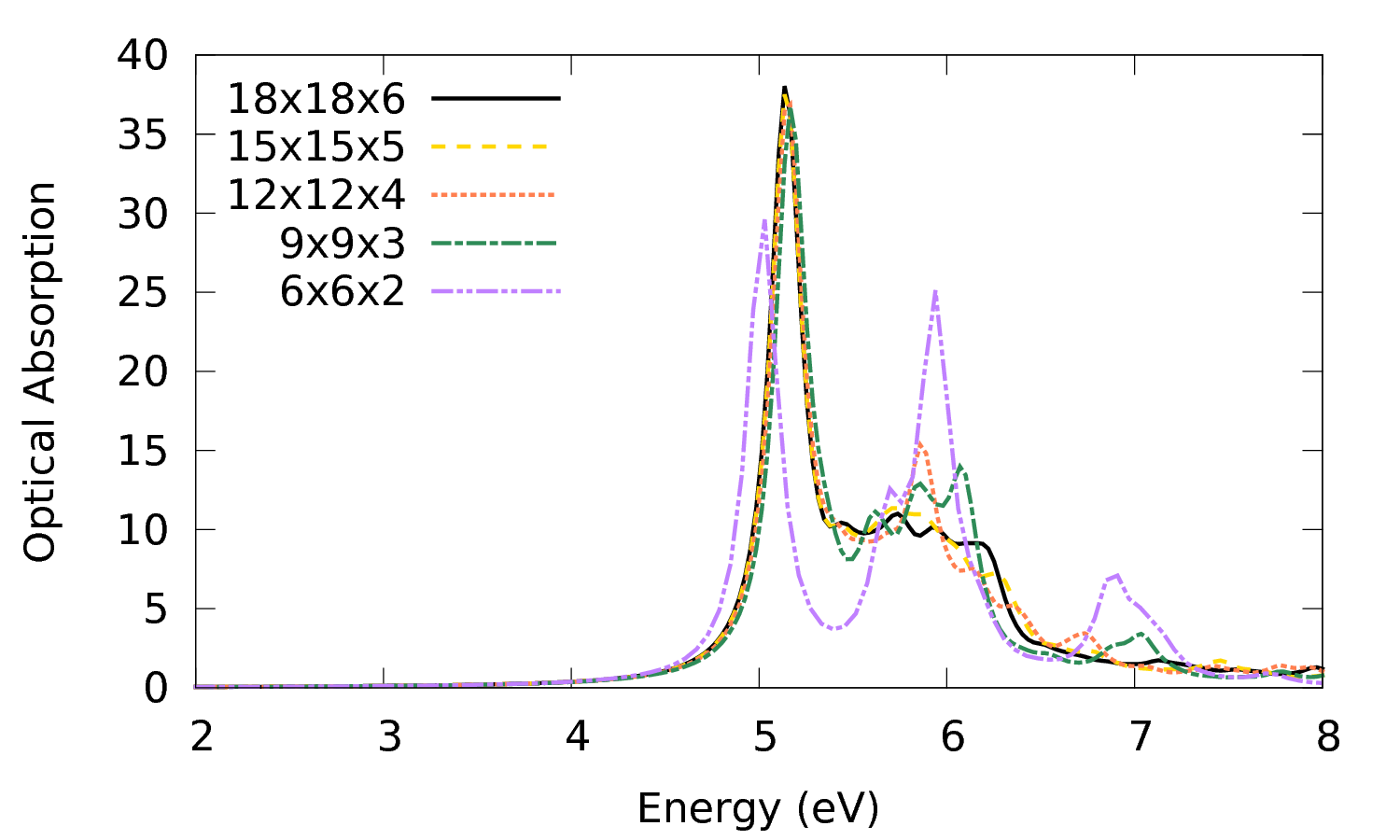
To see the effect of k-points plot those files with gnuplot (remember to include the 6x6x2 calculation which should still be inside hBN/YAMBO, if the parameters don't match you simply rerun it here by creating a 6x6x2 directory and copying the SAVE there):
> gnuplot
plot '18x18x6/o-3D_18186.eps_q1_haydock_bse' w l t '18x18x6, '15x15x5/o-3D_15155.eps_q1_haydock_bse' w l t '15x15x5','12x12x4/o-3D_12124.eps_q1_haydock_bse' w l t '12x12x4,
'9x9x3/o-3D_993.eps_q1_haydock_bse' w l t '9x9x3', '6x6x2/o-3D_662.eps_q1_haydock_bse' w l t '6x6x2'
From this plot you can notice that:
- results with the 6x6x2 mesh are clearly not converged: the first peak is too red shifted, the peak at 6 eV too sharp and intense and there is an 'extra' peak at 7 eV.
- both the position and shape of the first peak are practically converged with the 9x9x3 mesh.
- conversely the second peak is still not fully converged with the 18x18x6.
The different behavior in the convergence of the two features depends on the localization of the exciton. The sharp first peak suggests a localized exciton. The shape of the second peak a much more delocalized exciton. A finer k mesh, corresponds in direct space, to considering a larger amount of unit cells. Then when the excitation is delocalized over a large number of unit cells a very fine k mesh is needed. Typically a too coarse k mesh induces an artificial localization of the excitons which then correspond to artefacts in the spectrum (similar to what is observed for the 6x6x9). A nice, instructive discussion on wrong deductions from unconverged k mesh calculations can be found in the Appendix of Molina-Sanchez et al. (2013).[1]
Summary
To sum-up the results from this tutorial you have found that for the system under study:
BSENGBlk= 3 RyBSENGexx= 10 RyBSEBands from 6 to 10- To converge the position and shape of the first exciton peak a 12x12x4 mesh is sufficient. For the second exciton peak a mesh larger than 18x18x6 would be needed (indeed Wirtz and co-workers found a k-mesh 24x24x10 was needed.[2])
Links
- Go to Calculating optical spectra including excitonic effects: a step-by-step guide module
- Back to Modena 2025
- Back to Rome 2023#Tutorials
- Back to BSE tutorial sections
- Back to ICTP 2022
- Back to CECAM VIRTUAL 2021
- Back to technical modules menu
- Back to tutorials menu
