Local fields: Difference between revisions
(→Links) |
No edit summary |
||
| Line 1: | Line 1: | ||
In this | In this module you will learn how to calculate the macroscopic dielectric function in 2D hBN. | ||
== Background == | == Background == | ||
The macroscopic dielectric function is obtained by including the so-called local field effects (LFE) in the calculation of the response function. Within the time-dependent DFT formalism this is achieved by solving the Dyson equation for ''X''. In reciprocal space this is given by: | The macroscopic dielectric function is obtained by including the so-called local field effects (LFE) in the calculation of the response function. Within the time-dependent DFT formalism this is achieved by solving the Dyson equation for the susceptibility ''X''. In reciprocal space this is given by: | ||
[[File:Yambo-CH7.png|none|x50px|Yambo tutorial image]] | [[File:Yambo-CH7.png|none|x50px|Yambo tutorial image]] | ||
The microscopic dielectric function is related to ''X'' by: | The microscopic dielectric function is related to ''X'' by: | ||
| Line 10: | Line 10: | ||
[[File:Yambo-CH8.png|none|x60px|Yambo tutorial image]] | [[File:Yambo-CH8.png|none|x60px|Yambo tutorial image]] | ||
In the following we will neglect the ''f <sup> xc</sup>'' term: we perform the calculation at the RPA level and consider just the Hartree term in the | In the following we will neglect the ''f <sup> xc</sup>'' term: we perform the calculation at the RPA level and consider just the Hartree term in the kernel. | ||
== Prerequisites == | == Prerequisites == | ||
* You must first complete the "How to use Yambo" | * You must first complete the "How to use Yambo" modules | ||
'''You will need''': | '''You will need''': | ||
| Line 24: | Line 24: | ||
Enter the folder for 2D hBN that contains the SAVE directory, and generate the input file. From <code>yambo -H</code> you should understand that the correct option is <code>yambo -o c -k hartree</code>. Let's start by running the calculation for light polarization ''q'' in the plane of the BN sheet: | Enter the folder for 2D hBN that contains the SAVE directory, and generate the input file. From <code>yambo -H</code> you should understand that the correct option is <code>yambo -o c -k hartree</code>. Let's start by running the calculation for light polarization ''q'' in the plane of the BN sheet: | ||
$ cd YAMBO_TUTORIALS/hBN-2D/YAMBO | $ cd YAMBO_TUTORIALS/hBN-2D/YAMBO | ||
$ yambo. ''(Initialization)'' | |||
$ yambo -F yambo.in_RPA -V RL -J q100 -o c -k hartree | $ yambo -F yambo.in_RPA -V RL -J q100 -o c -k hartree | ||
and make sure to set/modify all of the following variables to: | and make sure to set/modify all of the following variables to: | ||
| Line 45: | Line 46: | ||
* A ''q'' parallel to the sheet | * A ''q'' parallel to the sheet | ||
* A wider energy range than before, and more broadening | * A wider energy range than before, and more broadening | ||
* Selected the Hartree kernel, and | * Selected the Hartree kernel, and expanded G-vectors in the screening up to 3 Ry (about 85 G-vectors) | ||
==LFEs in periodic direction== | ==LFEs in periodic direction== | ||
| Line 74: | Line 75: | ||
gnuplot> plot "o-q001.eps_q1_inv_rpa_dyson" u 1:2 w l,"o-q001.eps_q1_inv_rpa_dyson" u 1:4 w l | gnuplot> plot "o-q001.eps_q1_inv_rpa_dyson" u 1:2 w l,"o-q001.eps_q1_inv_rpa_dyson" u 1:4 w l | ||
[[File:CH-LFE6.png|none|600px|Yambo tutorial image]] | [[File:CH-LFE6.png|none|600px|Yambo tutorial image]] | ||
In this case, the absorption is strongly blueshifted. Furthermore, the influence of local fields is striking, and quenches the spectrum strongly. | In this case, the absorption is strongly blueshifted with respect to the in plane absorption. Furthermore, the influence of local fields is striking, and quenches the spectrum strongly. This is the well known depolarization effect. | ||
==Absorption versus EELS== | ==Absorption versus EELS== | ||
In order to understand this, we plot the electron energy loss spectrum for this component and compare with the absorption: | In order to understand this further, we plot the electron energy loss spectrum for this component and compare with the absorption: | ||
$ gnuplot | $ gnuplot | ||
gnuplot > plot "o-q001.eps_q1_inv_rpa_dyson" w l,"o-q001.eel_q1_inv_rpa_dyson" w l | gnuplot > plot "o-q001.eps_q1_inv_rpa_dyson" w l,"o-q001.eel_q1_inv_rpa_dyson" w l | ||
Revision as of 17:16, 30 March 2017
In this module you will learn how to calculate the macroscopic dielectric function in 2D hBN.
Background
The macroscopic dielectric function is obtained by including the so-called local field effects (LFE) in the calculation of the response function. Within the time-dependent DFT formalism this is achieved by solving the Dyson equation for the susceptibility X. In reciprocal space this is given by:
The microscopic dielectric function is related to X by:
and the macroscopic dielectric function is obtained by taking the (0,0) component of the inverse microscopic one:
Experimental observables like the optical absorption and the electron energy loss can be obtained from the macroscopic dielectric function:
In the following we will neglect the f xc term: we perform the calculation at the RPA level and consider just the Hartree term in the kernel.
Prerequisites
- You must first complete the "How to use Yambo" modules
You will need:
- The
SAVEdatabases for 2D hBN - The
yamboexecutable gnuplotfor plotting spectra
Choosing input parameters
Enter the folder for 2D hBN that contains the SAVE directory, and generate the input file. From yambo -H you should understand that the correct option is yambo -o c -k hartree. Let's start by running the calculation for light polarization q in the plane of the BN sheet:
$ cd YAMBO_TUTORIALS/hBN-2D/YAMBO
$ yambo.       (Initialization)
$ yambo -F yambo.in_RPA -V RL -J q100 -o c -k hartree
and make sure to set/modify all of the following variables to:
FFTGvecs=     6        Ry    # [FFT] Plane-waves
Chimod= "Hartree"            # [X] IP/Hartree/ALDA/LRC/BSfxc
NGsBlkXd=     3        Ry    # [Xd] Response block size
% QpntsRXd
 1 |  1 |                   # [Xd] Transferred momenta
%
% EnRngeXd
 0.00000 | 20.00000 | eV    # [Xd] Energy range
%
% DmRngeXd
0.200000 | 0.200000 | eV    # [Xd] Damping range
%
ETStpsXd= 2001               # [Xd] Total Energy steps
% LongDrXd
1.000000 | 0.000000 | 0.000000 |        # [Xd] [cc] Electric Field
%
In this input file, we have:
- A q parallel to the sheet
- A wider energy range than before, and more broadening
- Selected the Hartree kernel, and expanded G-vectors in the screening up to 3 Ry (about 85 G-vectors)
LFEs in periodic direction
Now let's run the code with this new input file:
$ yambo -F yambo.in_RPA -V RL -J q100
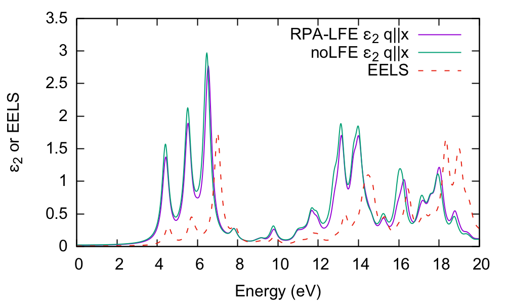
and let's compare the absorption with and without the local fields included. By inspecting the o-q100.eps_q1_inv_rpa_dyson file we find that this information is given in the 2nd and 4th columns, respectively:
$ head -n30 o-q100.eps_q1_inv_rpa_dyson
# Absorption @ Q(1) [q->0 direction] : 1.0000000  0.0000000  0.0000000
#  E/ev[1]     EPS-Im[2]   EPS-Re[3]   EPSo-Im[4]  EPSo-Re[5]
Plot the result:
$ gnuplot
gnuplot> plot "o-q100.eps_q1_inv_rpa_dyson" u 1:2 w l,"o-q100.eps_q1_inv_rpa_dyson" u 1:4 w l
It is clear that there is little influence of local fields in this case. We have also shown the EELS spectrum (o-q100.eel_q1_inv_rpa_dyson) for comparison.
LFEs in non-periodic direction
Now let's switch to q perpendicular to the BN plane:
$ yambo -F yambo.in_RPA -V RL -J q001 -o c -k hartree        and set
...
% LongDrXd
0.000000 | 0.000000 | 1.000000 |        # [Xd] [cc] Electric Field
%
...
$ yambo -F yambo.in_RPA -V RL -J q001
Plotting the output file:
$ gnuplot
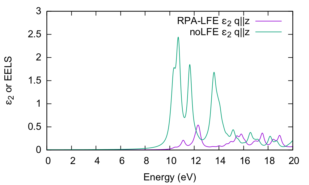
gnuplot> plot "o-q001.eps_q1_inv_rpa_dyson" u 1:2 w l,"o-q001.eps_q1_inv_rpa_dyson" u 1:4 w l
In this case, the absorption is strongly blueshifted with respect to the in plane absorption. Furthermore, the influence of local fields is striking, and quenches the spectrum strongly. This is the well known depolarization effect.
Absorption versus EELS
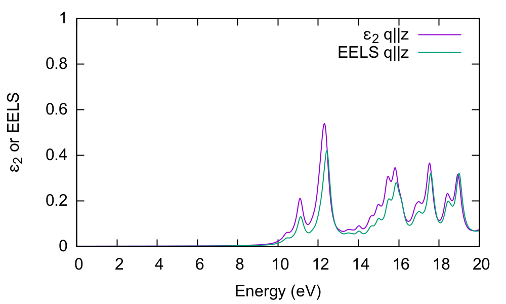
In order to understand this further, we plot the electron energy loss spectrum for this component and compare with the absorption:
$ gnuplot
gnuplot > plot "o-q001.eps_q1_inv_rpa_dyson" w l,"o-q001.eel_q1_inv_rpa_dyson" w l
The conclusion is that the dielectric function and EELS coincide for isolated systems. You should verify that this is not the case for the periodic (in-plane) direction.
Summary
From this tutorial you've learned:
- How to compute the macroscopic dielectric function by solving the Dyson equation for X in G-space
- The connection between absorption and EELS in low-dimensional systems
Links
- Previous module: Optics at the independent particle level
- Back to First steps with yambo tutorial
- Back to tutorials menu


