How to analyse excitons

In this tutorial you will learn (for a 2D-hBN) how to:

• How to analyze a BSE optical spectrum in terms of excitonic eigenvectors and eigenvalues
• How to plot the excitonic wavefunction

Prerequisites

Previous modules

• You must have completed the tutorial on 2D hBN.
• You must have completed the tutorial on 2D hBN.

You will need:

• ypp executable
• xcrysden executable
• gnuplot or xmgrace executable

YAMBO calculations

If you have completed the tutorial you should have all the databases required to do this tutorial in your SAVE and 2D directories

$ ls ./SAVE
ndb.gops			ns.kb_pp_pwscf_fragment_2	ns.kb_pp_pwscf_fragment_7	ns.wf_fragments_4_1
ndb.kindx			ns.kb_pp_pwscf_fragment_3	ns.wf				ns.wf_fragments_5_1
ns.db1				ns.kb_pp_pwscf_fragment_4	ns.wf_fragments_1_1		ns.wf_fragments_6_1
ns.kb_pp_pwscf			ns.kb_pp_pwscf_fragment_5	ns.wf_fragments_2_1		ns.wf_fragments_7_1
ns.kb_pp_pwscf_fragment_1	ns.kb_pp_pwscf_fragment_6	ns.wf_fragments_3_1
$ ls ./2D
ndb.BS_Q1_CPU_0			ndb.dip_iR_and_P		ndb.dip_iR_and_P_fragment_6	ndb.pp_fragment_4
ndb.BS_diago_Q01		ndb.dip_iR_and_P_fragment_1	ndb.dip_iR_and_P_fragment_7	ndb.pp_fragment_5
ndb.HF_and_locXC		ndb.dip_iR_and_P_fragment_2	ndb.pp				ndb.pp_fragment_6
ndb.QP				ndb.dip_iR_and_P_fragment_3	ndb.pp_fragment_1		ndb.pp_fragment_7
ndb.RIM				ndb.dip_iR_and_P_fragment_4	ndb.pp_fragment_2
ndb.cutoff			ndb.dip_iR_and_P_fragment_5	ndb.pp_fragment_3

Postprocessing calculations

$ ypp -e -s -J 2D 

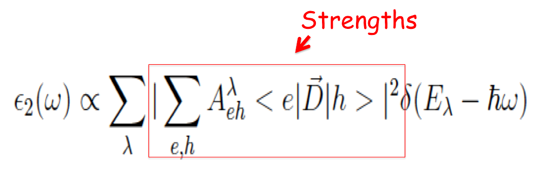
The new generated file o-2D.exc_E_sorted (o-2D.exc_E_sorted) reports the energies of the excitons and their Dipole Oscillator Strenghts sorted by energy (Index).

Open one of them and have look inside.