Modena 2025 : Yambopy part 2

In this tutorial we will first plot and interpolate GW band structures calculated with YAMBO, then deal with the analysis of excitons from a BSE calculation.

Make sure you have completed Modena 2025: Yambopy part 1 and have the relevant databases in your $SCRATCH directory.

cd $SCRATCH
cd YAMBOPY_TUTORIALS

GW calculations

Tutorial 1: GW bands

Yambopy can be used either to run Yambo and QE calculations, or to analyse the results of QE and Yambo by dealing with their generated databases. This is done with a variety of classes included in the qepy (for QE) or yambopy (for Yambo) modules. In the case of Yambo GW quasi-particle calculations, we can use the yambopy class YamboQPDB to read the database produced by the simulation. Enter in the folder

cd databases_qepy/gw-bands

We can use this to find the scissor operator, plot the GW bands and to interpolate the GW bands on a smoother k-path. The example runs by typing:

python plot-qp.py

See below for an explanation of the tutorial. As usual, we can import the qepy and yambopy libraries:

 from yambopy import YamboLatticeDB,YamboQPDB
 from qepy import Path

We define the k-points path.

 npoints = 10
 path = Path([ [[  0.0,  0.0,  0.0],'$\Gamma$'],
               [[  0.5,  0.0,  0.0],'M'],
               [[1./3.,1./3.,  0.0],'K'],
               [[  0.0,  0.0,  0.0],'$\Gamma$']], [int(npoints*2),int(npoints),int(sqrt(5)*npoints)] )

Importantly, the number of points is a free choice used only in case of interpolation. We can increase the variable npoints as we wish, it just means that the interpolation step will take more time. In order to analyse GW results we need to have the file related to the basic data of our Yambo calculation (SAVE/ns.db1) and the netcdf file with the quasi-particle results (ndb.QP). We load the data calling the respective classes:

# Read Lattice information from SAVE
lat  = YamboSaveDB.from_db_file(folder='SAVE',filename='ns.db1')
# Read QP database
ydb  = YamboQPDB.from_db(filename='ndb.QP',folder='qp-gw')

(as you know by now, in the yambopy module each class is specialised to read a specific Yambo database)

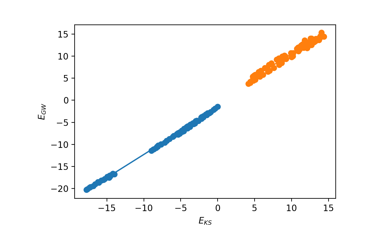
The first option is to plot the energies and calculate the ideal Kohn-Sham to GW scissor operator. We need to select the index of the top valence band:

n_top_vb = 4
ydb.plot_scissor_ax(ax,n_top_vb)

Yambopy displays the fitting and also the data of the slope of each fitting. Notice that this is also a test if the GW calculations are running well. If the dependence is not approaching linear you should double-check your results!

In this case the slope is:

valence bands:
slope:     1.0515886598785766
conduction bands:
slope:     1.026524081134514
scissor list (shift,c,v) [eV,adim,adim]: [1.8985204833551723, 1.026524081134514, 1.0515886598785766]

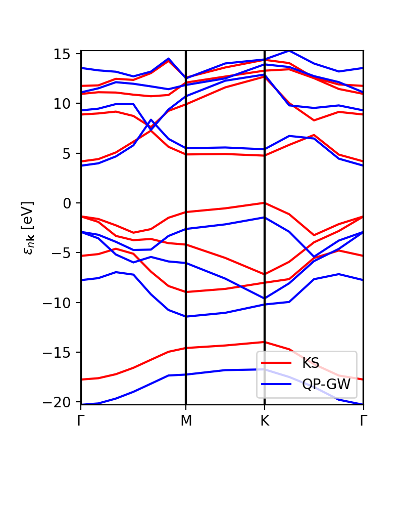
In addition to the scissor operator, we can plot the GW (and DFT) band structure along the path. The first choice would be to plot the actual GW calculations, without interpolation, to check that the results are meaningful (or not). This plot is independent of the number of k-points (npoints) that we want to put in the interpolation. The class YamboQPDB finds the calculated points that belong to the path and plots them. Be aware that if we use coarse grids the class would not find any point and the function will not work.

ks_bs_0, qp_bs_0 = ydb.get_bs_path(lat,path)
ks_bs_0.plot_ax(ax,legend=True,c_bands='r',label='KS')
qp_bs_0.plot_ax(ax,legend=True,c_bands='b',label='QP-GW')

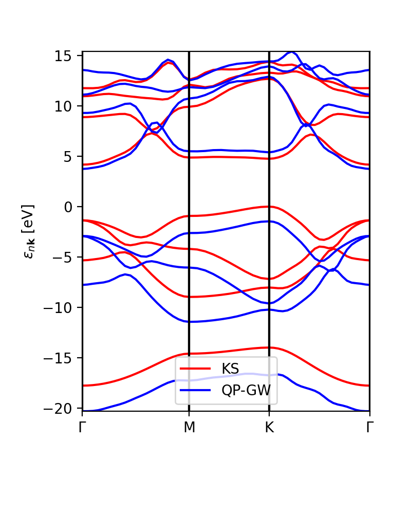
The interpolation of the DFT and GW band structures looks similar:

ks_bs, qp_bs = ydb.interpolate(lat,path,what='QP+KS',lpratio=20)
ks_bs.plot_ax(ax,legend=True,c_bands='r',label='KS')
qp_bs.plot_ax(ax,legend=True,c_bands='b',label='QP-GW')

The lpratio can be increased if the interpolation does not work as well as intended. The SKW interpolation scheme is the same one implemented in abipy (the python interface for the Abinit DFT code).

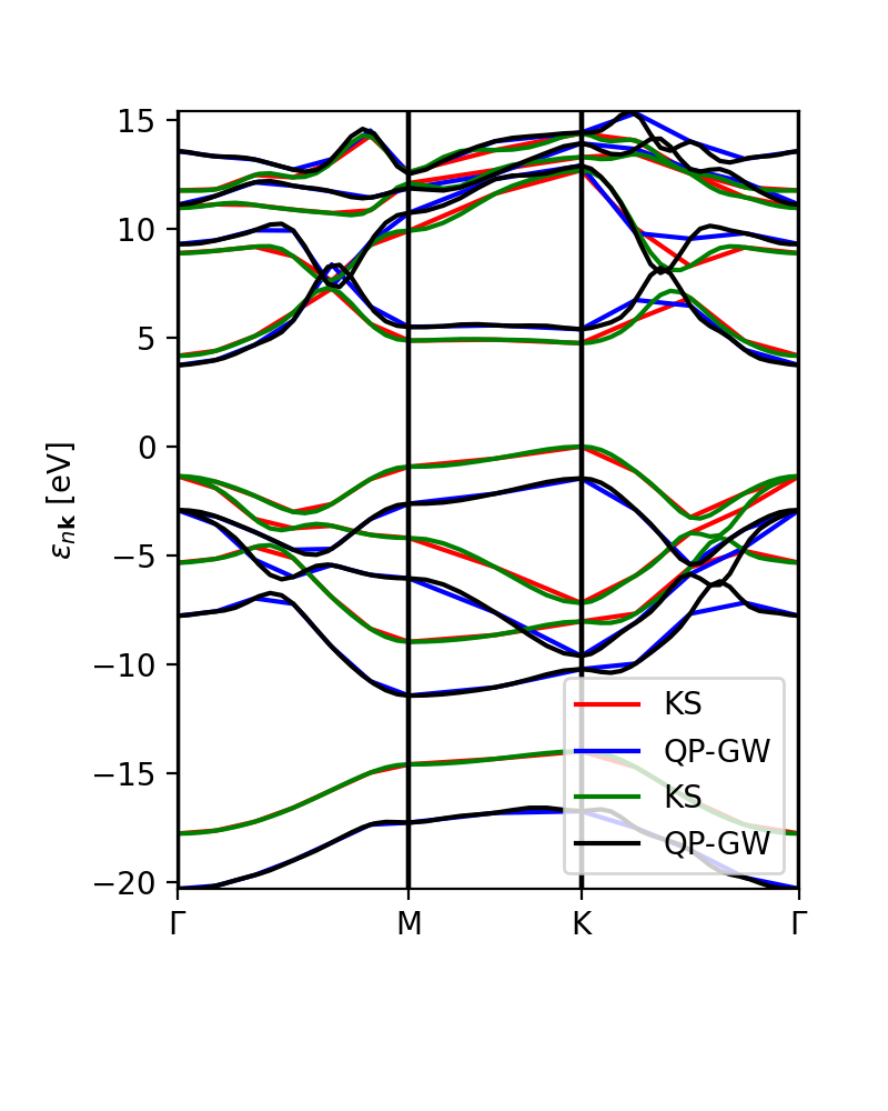
Finally, we can compare the calculated GW eigenvalues with the interpolation.

Excitons

Let us now move to the directory where the exciton data for the next tutorials are stored:

cd ../../databases_yambopy

Tutorial 2: read and sort exciton data

In this section we will use the script exc_read.py and read the exciton data resulting from a BSE calculation in order to familiarise with their structure. This time we are going to read the ndb.BS_diago_Q* databases which correspond to BSE calculations at various momenta Q (Q=1 being the zero-momentum optical absorption limit - notice that python indexing starts from 0, while the databases are counted starting from 1).

In order to read them in python we use the Yambopy class YamboExcitonDB, which can be instanced like this:

yexc = YamboExcitonDB.from_db_file(ylat,filename=f'path/to/BSE/databases/ndb.BS_diago_Q{i}')

(where i is the number of BS_diago_Qi file. Notice that it requires a previous instance of YamboLatticeDB).

Now the yexc object contains information about the exciton energies (yexc.eigenvalues), wave functions (yexc.eigenvectors) and intensities (yexc.l_residuals, yexc.r_residuals) for Qpoint i_Q. You can start by keeping Q1 which is the optical limit and then check other momenta.

The exciton wave function components A_{vck}^{\lambda Q} (\lambda being the exciton index) are stored as A_{t}^{\lambda} in each Q-dependent database, with t being the transition index grouping the single-particle indices vck. Therefore, yexc.eigenvectors is an array with (N_excitons,N_transitions) dimension. In order to make the connection t->kcv, the table yexc.table provides k,v,c and spin indices corresponding to each transition.

In order to get a clearer picture, take a look at the script exc_read.py. Run it and try to understand the outputs.

 python exc_read.py

Tutorial 3: plot exciton weights on k-BZ and (interpolated) band structure

In this section we will use the script exc_kspace_plot.py and work with the quantities defined in the previous section.

We will focus on the i_Q=0 case (the optical limit). We want to check the relative importance of the various (vk->ck) electronic transitions in forming a certain excitonic state.

Since many excitonic states are degenerate, we first need to tell Yambopy which states we want to check. For example, in monolayer hexagonal boron nitride, the lowest-bound exciton - forming the main peak in the BSE absorption spectrum - is doubly degenerate. In order to analyse it, in the exc_kspace_plot.py script we set

states = [1,2]

(we can also set [3,4] to check the second excitonic state, and then [5] for the non-degenerate third state, and so on; we can check degeneracies by printing the energies using the script exc_read.py).

In order to make a band structure plot, it is necessary to read the band energies with the YamboElectronsDB class

yel = YamboElectronsDB.from_db_file(folder='path/to/SAVE')

and specify the path in the BZ using crystal coordinates via the Path function:

npoints = 20
path = Path([ [[  0.0,  0.0,  0.0],'$\Gamma$'],
              [[  0.5,  0.0,  0.0],'M'],
              [[1./3.,1./3.,  0.0],'K'],
              [[  0.0,  0.0,  0.0],'$\Gamma$']],
              [int(npoints*2),int(npoints),int(sqrt(5)*npoints)] )

Now let's take a closer look at the exc_kspace_plot.py script. You will see that it performs three plots:

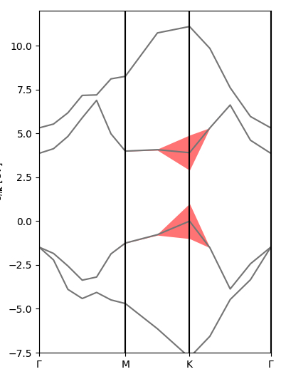
• Plot of |A(k)| in the k-BZ for the selected exciton state. You can see how most contributions come from the area around K and the MK direction [Kspace_Plot=True].
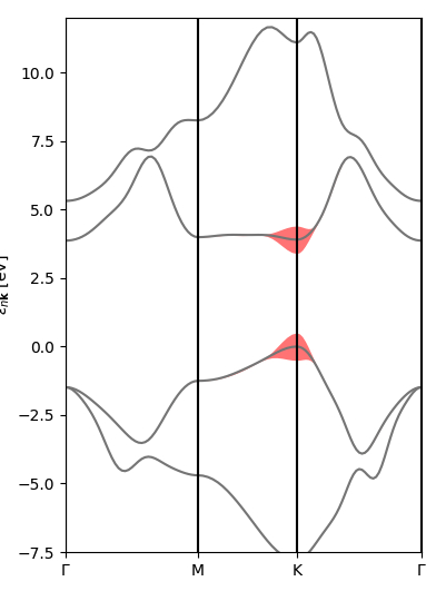
• Plot of |A(v,c,k)| on the electronic band structure for the selected exciton state. Here you can better see how the top valence and bottom conduction around MK are mostly involved [Bands_Plot=True].
• Plot of interpolated |A(v,c,k)| on the interpolated electronic band structure for the selected exciton state [Bands_Plot_Interpolated=True].

As always, try to play with the parameters, for example by changing the excitonic states to analyse.

Tutorial 4: plot BSE optical absorption with custom options

In this section we will use the script exc_abs_plot.py and work with the quantities defined in the previous sections.

The class YamboExcitonDB also enables us, of course, to read the dielectric function eps(w) and print absorption and related spectra in python.

The advantages over using the standard human-readable yambo outputs are mainly two:

1. We can freely select energy ranges, energy steps, peak broadenings and number of excitonic states included without having to rerun the yambo executable every time. This reduces the chance of mistakenly editing the yambo input and allows for greater freedom since these plots can now be done in your local machine without having to transfer the output data from a remote cluster.
2. The dielectric function constructed from netCDF database variables has a much higher precision (number of significant digits) than the human readable output, which may be important if you want to perform additional operations in python (e.g., computing refractive index, reflectivity and other optical spectra from it, performing finite-difference derivatives, etc).

We can read eps(w) as a numpy array with the specified options as (energy values are in eV):

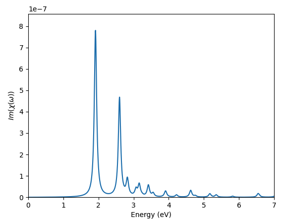
w, eps = yexc.get_chi(nexcitons='all',emin=0,emax=7,estep=0.005,broad=0.04)

Or, you can directly prepare a plot of its imaginary part with

w, chi = yexc.plot_chi_ax(ax,nexcitons='all',emin=0,emax=7,estep=0.005,broad=0.04)

where ax is a previously defined Axes object from matplotlib.

In order to see how this works, let's take a look at the exc_abs_plot.py script. You will see that it performs the two operations described above:

• Plotting the BSE absorption spectrum [Absorption_Plot=True].
• Reading the complex dielectric function.

Try to customise the plots by changing the nexcitons, emin, emax, estep, broad parameters.

Links

• Back to Modena 2025 : Yambopy part 1
• Back to Modena 2025