Shift current: Difference between revisions
No edit summary |
|||
| (9 intermediate revisions by the same user not shown) | |||
| Line 29: | Line 29: | ||
OSCLL_Threads=0 # [OPENMP/X] Number of threads for Oscillators | OSCLL_Threads=0 # [OPENMP/X] Number of threads for Oscillators | ||
% NLBands | % NLBands | ||
<span style="color:red">3 | | <span style="color:red">3 | 5 | </span> # [NL] Bands range | ||
% | % | ||
NLverbosity= "high" # [NL] Verbosity level (low | high) | NLverbosity= "high" # [NL] Verbosity level (low | high) | ||
| Line 37: | Line 37: | ||
NLLrcAlpha= 0.000000 # [NL] Long Range Correction | NLLrcAlpha= 0.000000 # [NL] Long Range Correction | ||
% NLEnRange | % NLEnRange | ||
<span style="color:red"> 1.000000 | | <span style="color:red"> 1.000000 | 8.000000 </span> | eV # [NL] Energy range (for loop on frequencies NLEnSteps/=0 | ||
% | % | ||
NLEnSteps= <span style="color:red"> | NLEnSteps= <span style="color:red">48 </span> # [NL] Energy steps for the loop on frequencies | ||
% NLrotaxis | % NLrotaxis | ||
0.000000 | 0.000000 | 0.000000 | # [NL] Rotation axis (for the loop on angles NLAngSteps/=0) | 0.000000 | 0.000000 | 0.000000 | # [NL] Rotation axis (for the loop on angles NLAngSteps/=0) | ||
| Line 62: | Line 62: | ||
Notice that in this input we turned one the evaluation of current <span style="color:red">EvalCurrent</span> and force the parallelization on the frequencies, <br><code>NL_CPU= " <span style="color:red">8 1</span></code>, <code> NL_ROLEs= " <span style="color:red">w k</span> </code>, that is much more efficient than the one on k-points. | Notice that in this input we turned one the evaluation of current <span style="color:red">EvalCurrent</span> and force the parallelization on the frequencies, <br><code>NL_CPU= " <span style="color:red">8 1</span></code>, <code> NL_ROLEs= " <span style="color:red">w k</span> </code>, that is much more efficient than the one on k-points. | ||
== Analysis of the results == | |||
In order to analyze the result we use the branch '''shift_current''' of this Yambopy: [https://github.com/attacc/yambopy/tree/shift_current https://github.com/attacc/yambopy/tree/shift_current],<br> and the following script for the post-processing: | |||
from yambopy import * | |||
from yambopy.nl.harmonic_analysis import Harmonic_Analysis | |||
from yambopy.units import fs2aut | |||
X_order=4 | |||
NLDB=YamboNLDB() | |||
Harmonic_Analysis(NLDB,X_order=X_order,prn_Peff=True) | |||
Then you can plot the file <code>o.YamboPy-Sigma_probe_order_0</code> that contains the DC part of the current. In the figure below I plot the 5th column<br> | |||
that corresponds to the real part of <math>\sigma^{yyy}</math>: | |||
[[File:Sigma2.png|center| 600px | Shift current]] | |||
Then we used this script to plot the result: | |||
import matplotlib.pyplot as plt | |||
import numpy as np | |||
fig = plt.figure(figsize=(10,10)) | |||
ax = fig.add_subplot() | |||
plt.title("$|\sigma^{(2)}(0,\omega_1-\omega_1$)|",fontsize=20) | |||
fontsize2=14 | |||
XHI0 = np.genfromtxt('o.YamboPy-Sigma_probe_order_0',comments="#") | |||
plt.tick_params(\ | |||
axis='x', # changes apply to the x-axis | |||
which='both', # both major and minor ticks are affected | |||
bottom='off', # ticks along the bottom edge are off | |||
top='off', # ticks along the top edge are off | |||
labelbottom='off') | |||
plt.xlim(1.0,7.5) | |||
plt.xlabel('Energy [eV]',fontsize=20) | |||
plt.tick_params(axis='y', which='major', labelsize=14) | |||
# plt.plot(XHI0[:,0], XHI0[:,2], linewidth=2.5, linestyle="-",label='$\sigma^{(xyy)}$') | |||
plt.plot(XHI0[:,0], XHI0[:,4], linewidth=2.5, linestyle="-",label='Re $\sigma^{(yyy)}$') | |||
plt.axhline(y=0.0, color='black', linestyle='-') | |||
plt.legend(loc="upper right",fontsize=fontsize2) | |||
plt.xticks(fontsize=fontsize2) | |||
plt.savefig('sigma2.png', format='png') | |||
plt.show() | |||
Latest revision as of 14:50, 29 August 2024
This tutorial is for internal use only, these response functions are not implemented/tested in yambo/yambopy suite.
Introduction
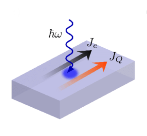
In this tutorial we will show how to calculate Shift Current in bulk materials.
We suppose you are already familiar with the non-linear response using the Yambo code.
If it is not the case please study the previous tutorials:
Linear response using Dynamical Berry Phase and Real time approach to non-linear response (SHG).
Setup calculations
In this tutorial we will take as example the two dimensional hBN.
DFT wave-functions and inputs can be downloaded here: hBN-2D-RT.tar.gz.
First of all run the setup, then remove symmetries along the y direction, as explained in the tutorial above.
Real-time setup and calculations
In order to generate input file for shift current you do: yambo_nl -u n -V par
nloptics                         # [R] Non-linear spectroscopy
NLogCPUs=0                       # [PARALLEL] Live-timing CPU`s (0 for all)
PAR_def_mode= "balanced"         # [PARALLEL] Default distribution mode ("balanced"/"memory"/"workload"/"KQmemory")
NL_CPU= " 8 1"                       # [PARALLEL] CPUs for each role
NL_ROLEs= " w k"                     # [PARALLEL] CPUs roles (w,k)
DIP_CPU= ""                      # [PARALLEL] CPUs for each role
DIP_ROLEs= ""                    # [PARALLEL] CPUs roles (k,c,v)
OSCLL_CPU= ""                    # [PARALLEL] CPUs for each role
OSCLL_ROLEs= ""                  # [PARALLEL] CPUs roles (k,b)
DIP_Threads=0                    # [OPENMP/X] Number of threads for dipoles
NL_Threads=0                     # [OPENMP/NL] Number of threads for nl-optics
OSCLL_Threads=0                  # [OPENMP/X] Number of threads for Oscillators
% NLBands
  3 |  5 |                           # [NL] Bands range
%
NLverbosity= "high"              # [NL] Verbosity level (low | high)
NLtime=-1.000000           fs    # [NL] Simulation Time
NLintegrator= "INVINT"           # [NL] Integrator ("EULEREXP/RK2/RK4/RK2EXP/HEUN/INVINT/CRANKNIC")
NLCorrelation= "IPA"             # [NL] Correlation ("IPA/HARTREE/TDDFT/LRC/LRW/JGM/SEX/LSEX/LHF")
NLLrcAlpha= 0.000000             # [NL] Long Range Correction
% NLEnRange
 1.000000 | 8.000000  |         eV    # [NL] Energy range (for loop on frequencies NLEnSteps/=0
%
NLEnSteps=  48                    # [NL] Energy steps for the loop on frequencies
% NLrotaxis
 0.000000 | 0.000000 | 0.000000 |        # [NL] Rotation axis (for the loop on angles NLAngSteps/=0)
%
NLAngSteps=0                     # [NL] Angular steps (if NLAngSteps/=0 field versor will be ignored)
NLDamping= 0.200000        eV    # [NL] Damping (or dephasing)
RADLifeTime=-1.000000      fs    # [RT] Radiative life-time (if negative RADLifeTime=Phase_LifeTime)
EvalCurrent                    # [NL] Evaluate the current
#FrPolPerdic                   # [DIP] Force periodicity of polarization respect to the external field
% Field1_Freq
 0.100000 | 0.100000 |         eV    # [RT Field1] Frequency
%
Field1_NFreqs= 1                 # [RT Field1] Frequency
Field1_Int=  1000.00       kWLm2 # [RT Field1] Intensity
Field1_Width= 0.000000     fs    # [RT Field1] Width
Field1_kind= "SOFTSIN"           # [RT Field1] Kind(SIN|SOFTSIN| see more on src/modules/mod_fields.F)
Field1_pol= "linear"             # [RT Field1] Pol(linear|circular)
% Field1_Dir
 0.000000 | 1.000000 | 0.000000 |        # [RT Field1] Versor
%
Field1_Tstart= 0.010000    fs    # [RT Field1] Initial Time
Notice that in this input we turned one the evaluation of current EvalCurrent and force the parallelization on the frequencies, NL_CPU= " 8 1, NL_ROLEs= " w k , that is much more efficient than the one on k-points.
Analysis of the results
In order to analyze the result we use the branch shift_current of this Yambopy: https://github.com/attacc/yambopy/tree/shift_current,
and the following script for the post-processing:
from yambopy import *
from yambopy.nl.harmonic_analysis import Harmonic_Analysis
from yambopy.units import fs2aut
X_order=4
NLDB=YamboNLDB()
Harmonic_Analysis(NLDB,X_order=X_order,prn_Peff=True)
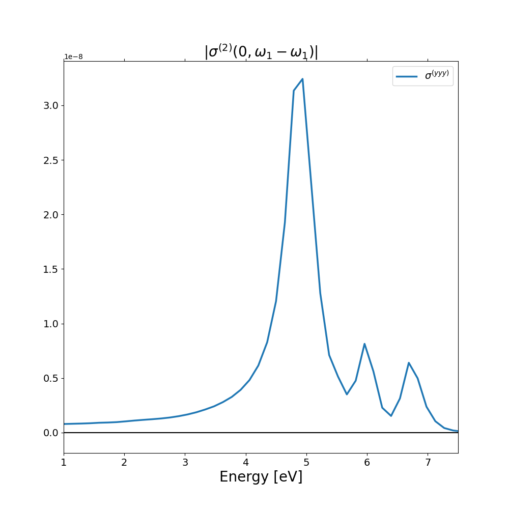
Then you can plot the file o.YamboPy-Sigma_probe_order_0 that contains the DC part of the current. In the figure below I plot the 5th column
that corresponds to the real part of [math]\displaystyle{ \sigma^{yyy} }[/math]:
Then we used this script to plot the result:
import matplotlib.pyplot as plt
import numpy as np
fig = plt.figure(figsize=(10,10))
ax = fig.add_subplot()
plt.title("$|\sigma^{(2)}(0,\omega_1-\omega_1$)|",fontsize=20)
fontsize2=14
XHI0 = np.genfromtxt('o.YamboPy-Sigma_probe_order_0',comments="#")
plt.tick_params(\
   axis='x',          # changes apply to the x-axis
   which='both',      # both major and minor ticks are affected
   bottom='off',      # ticks along the bottom edge are off
   top='off',         # ticks along the top edge are off
   labelbottom='off')
plt.xlim(1.0,7.5)
plt.xlabel('Energy [eV]',fontsize=20)
plt.tick_params(axis='y', which='major', labelsize=14)
# plt.plot(XHI0[:,0], XHI0[:,2], linewidth=2.5, linestyle="-",label='$\sigma^{(xyy)}$')
plt.plot(XHI0[:,0], XHI0[:,4], linewidth=2.5, linestyle="-",label='Re $\sigma^{(yyy)}$')
plt.axhline(y=0.0, color='black', linestyle='-')
plt.legend(loc="upper right",fontsize=fontsize2)
plt.xticks(fontsize=fontsize2)
plt.savefig('sigma2.png', format='png')
plt.show()

