Sum frequency generation

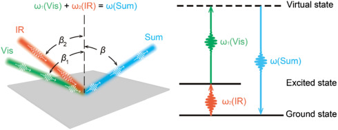
In this tutorial we will show how to calculate Sum Frequency Generation(SFG) and also Difference Frequency Generation (DFG) in bulk materials.
We suppose you are already familiar with the non-linear response using the Yambo code. If it is not the case please study the previous tutorials:
Linear response using Dynamical Berry Phase and Real time approach to non-linear response (SHG).

DFT calculations

In this example, we will consider a single layer of hexagonal boron nitride (hBN). If you didn't before you can download input files and Yambo databases for this tutorial here: hBN-2D-RT.tar.gz. and/or follow the instructions to generate the databases here: Prerequisites for Real Time propagation with Yambo

Removing symmetries

In this tutorial we will calculate the SFG along when both fields are in the 'y' direction, therefore we remove symmetries not compatible with an external field along this direction, with the command ypp_nl -y:

fixsyms                          # [R] Remove symmetries not consistent with an 
external perturbation
% Efield1
  0.000000 | 1.000000 | 0.000000 |        # First external Electric Field
%
% Efield2
 0.000000 | 0.000000 | 0.000000 |        # Additional external Electric Field
%
BField= 0.000000           T     # [MAG] Magnetic field modulus
Bpsi= 0.000000             deg   # [MAG] Magnetic field psi angle [degree]
Btheta= 0.000000           deg   # [MAG] Magnetic field theta angle [degree]
#RmAllSymm                     # Remove all symmetries
RmTimeRev                     # Remove Time Reversal
#RmSpaceInv                    # Remove Spatial Inversion

Real-time simulation with two external fields

You go in the FixSymm folder and run again the setup. Then you can put the following input file, that has been generated with the command  yambo_nl -u n , in the folder:

nloptics                         # [R] Non-linear spectroscopy
NLogCPUs=0                       # [PARALLEL] Live-timing CPU`s (0 for all)
PAR_def_mode= "balanced"         # [PARALLEL] Default distribution mode ("balanced"/"memory"/"workload"/"KQmemory")
NL_CPU= "10 1"                       # [PARALLEL] CPUs for each role
NL_ROLEs= "w k"                     # [PARALLEL] CPUs roles (w,k)
DIP_CPU= ""                      # [PARALLEL] CPUs for each role
DIP_ROLEs= ""                    # [PARALLEL] CPUs roles (k,c,v)
DIP_Threads=0                    # [OPENMP/X] Number of threads for dipoles
NL_Threads=0                     # [OPENMP/NL] Number of threads for nl-optics
% NLBands
  3 |  6 |                           # [NL] Bands range
%
NLverbosity= "low"              # [NL] Verbosity level (low | high)
NLtime= 60.00000           fs    # [NL] Simulation Time
NLintegrator= "CRANKNIC"         # [NL] Integrator ("EULEREXP/RK2/RK4/RK2EXP/HEUN/INVINT/CRANKNIC")
NLCorrelation= "IPA"             # [NL] Correlation ("IPA/HARTREE/TDDFT/LRC/LRW/JGM/SEX")
NLLrcAlpha= 0.000000             # [NL] Long Range Correction
% NLEnRange
 2.000000 | 8.000000 |         eV    # [NL] Energy range (for loop on frequencies NLEnSteps/=0
%
NLEnSteps= 30                   # [NL] Energy steps for the loop on frequencies
% NLrotaxis
 0.000000 | 0.000000 | 0.000000 |        # [NL] Rotation axis (for the loop on angles NLAngSteps/=0)
%
NLAngSteps=0                     # [NL] Angular steps (if NLAngSteps/=0 field versor will be ignored)
NLDamping= 0.200000        eV    # [NL] Damping (or dephasing)
RADLifeTime=-1.000000      fs    # [RT] Radiative life-time (if negative Yambo sets it equal to Phase_LifeTime in NL)
#EvalCurrent                   # [NL] Evaluate the current
#FrPolPerdic                   # [DIP] Force periodicity of polarization respect to the external field
HARRLvcs= 18475            RL    # [HA] Hartree     RL components
EXXRLvcs= 18475            RL    # [XX] Exchange    RL components
 % Field1_Freq
-0.100000 |-0.100000 |         eV    # [RT Field1] Frequency
%
Field1_NFreqs= 1                 # [RT Field1] Frequency
Field1_Int=  1000.00       kWLm2 # [RT Field1] Intensity
Field1_Width= 0.000000     fs    # [RT Field1] Width
Field1_kind= "SOFTSIN"           # [RT Field1] Kind(SIN|SOFTSIN| see more on src/modules/mod_fields.F)
Field1_pol= "linear"             # [RT Field1] Pol(linear|circular)
% Field1_Dir
 0.000000 | 1.000000 | 0.000000 |        # [RT Field1] Versor
%
Field1_Tstart= 0.010000    fs    # [RT Field1] Initial Time
% Field2_Freq
 2.000000 | 2.000000 |         eV    # [RT Field2] Frequency
%
Field2_NFreqs= 1                 # [RT Field2] Frequency
Field2_Int=  1000.00       kWLm2 # [RT Field2] Intensity
Field2_Width= 0.000000     fs    # [RT Field2] Width
Field2_kind= "SOFTSIN"           # [RT Field2] Kind(SIN|SOFTSIN| see more on src/modules/mod_fields.F)
Field2_pol= "linear"             # [RT Field2] Pol(linear|circular)
% Field2_Dir
 0.000000 | 1.000000 | 0.000000 |        # [RT Field2] Versor 
%
Field2_Tstart= 0.010000    fs    # [RT Field2] Initial Time

Analysis of the results