Linear response in velocity gauge: Difference between revisions
No edit summary |
|||
| (27 intermediate revisions by the same user not shown) | |||
| Line 1: | Line 1: | ||
[[File:Lresp.png|thumb|200px]] | [[File:Lresp.png|thumb|200px]] | ||
In this tutorial we show how to get the linear response using the velocity gauge instead of the Berry phase approach in length gauge. | In this tutorial we show how to get the linear response using the velocity gauge<br> instead of the Berry phase approach in length gauge.<br> | ||
We use the same input | We use the same DFT input files of the tutorial [[Linear response using Dynamical Berry Phase]], <br>run the same setup and remove the symmetries. | ||
<br> | |||
== Real-time dynamics in velocity gauge== | |||
Then in order to calculate the response in velocity gauge we use the command <code>yambo_nl -u p -V resp -F input_lr.in</code> to generate the input: | |||
nlinear # [R NL] Non-linear optics | |||
NL_Threads= 1 # [OPENMP/NL] Number of threads for nl-optics | |||
% NLBands | |||
<span style="color:red">3 | 6 | </span> # [NL] Bands | |||
% | |||
NLstep= <span style="color:red"> 0.0100 </span> fs # [NL] Real Time step length | |||
NLtime=55.000000 fs # [NL] Simulation Time | |||
NLintegrator= "INVINT" # [NL] Integrator ("EULEREXP/RK4/RK2EXP/HEUN/INVINT/CRANKNIC") | |||
NLCorrelation= "IPA" # [NL] Correlation ("IPA/HARTREE/TDDFT/LRC/JGM/SEX/HF") | |||
NLLrcAlpha= 0.000000 # [NL] Long Range Correction | |||
NLDamping= 0.000000 eV # [NL] Damping | |||
RADLifeTime=-1.000000 fs # [RT] Radiative life-time (if negative Yambo sets it equal to Phase_LifeTime in NL) | |||
#EvalCurrent # [NL] Evaluate the current | |||
#FrPolPerdic # [DIP] Force periodicity of polarization respect to the external field | |||
<span style="color:red">Gauge= "velocity" </span> # [BSE/X] Gauge (length|velocity) | |||
% Field1_Freq | |||
0.100000 | 0.100000 | eV # [RT Field1] Frequency | |||
% | |||
Field1_NFreqs= 1 # [RT Field1] Frequency | |||
Field1_Int= 1000.00 kWLm2 # [RT Field1] Intensity | |||
Field1_Width= 0.000000 fs # [RT Field1] Width | |||
Field1_kind= <span style="color:red"> "DELTA" </span> # [RT Field1] Kind(SIN|COS|RES|ANTIRES|GAUSS|DELTA|QSSIN) | |||
Field1_pol= "linear" # [RT Field1] Pol(linear|circular) | |||
% Field1_Dir | |||
<span style="color:red"> 0.000000 | 1.000000 | 0.000000 |</span> # [RT Field1] Versor | |||
% | |||
Field1_Tstart= 0.010000 fs # [RT Field1] Initial Time | |||
Notice that in velocity gauge the current is correct while the polarization is calculated using only intra-band dipoles, that anyway is enough for the linear response. | |||
==Analysis of the results using YamboPy using polarization == | |||
'''This part works only with Yambo 5.3 or the last version available on Github:''' [https://github.com/yambo-code/yambo https://github.com/yambo-code/yambo]<br> | |||
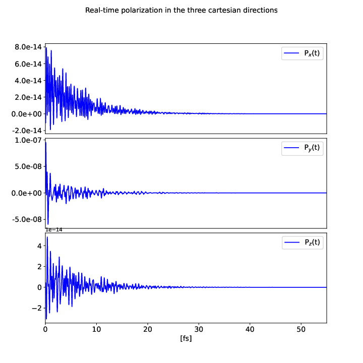
You can get the dielectric constant along the field direction using the same procedure of the Berry Phase case, Fourier transforming the polarization: | |||
import numpy as np | |||
from yambopy import * | |||
from yambopy.plot import * | |||
NLDB=YamboNLDB() | |||
pol =NLDB.Polarization[0] | |||
time=NLDB.IO_TIME_points | |||
t_initial=NLDB.Efield[0]["initial_time"] | |||
pol_damped=np.empty_like(pol) | |||
for i_d in range(3): | |||
pol_damped[i_d,:]=damp_it(pol[i_d,:],time,t_initial,damp_type='LORENTZIAN',damp_factor=0.1/ha2ev) | |||
Plot_Pol_or_Curr(time=time, pol=pol_damped, xlim=[0,55], save_file='polarization.pdf') | |||
[[File:Polarization velocity.png|center|Polarization_velocity]] | |||
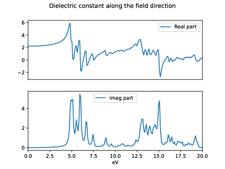
and then calculate the dielectric constant as in the length gauge | |||
Linear_Response(time=time,pol=-pol_damped,efield=NLDB.Efield[0],plot=False,plot_file='eps.pdf') | |||
notice that in this case, only the linear response along the field is correct. | |||
[[File:Eps velocity.png|center|Eps_velocity]] | |||
==Analysis of the results using YamboPy using current == | |||
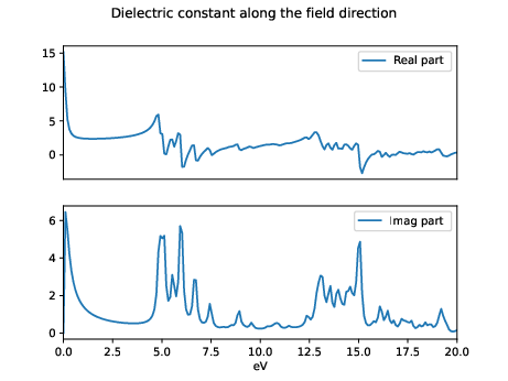
The same analysis can be performed using the current. <br>In this case we remove the constant term then we reconstruct the polarization | |||
and then the epsilon. | |||
import numpy as np | |||
from yambopy import * | |||
from yambopy.plot import * | |||
from scipy.interpolate import CubicSpline | |||
import matplotlib.pyplot as plt | |||
NLDB=YamboNLDB() | |||
current =NLDB.Current[0] | |||
time=NLDB.IO_TIME_points | |||
t_initial=NLDB.Efield[0]["initial_time"] | |||
# | |||
# Remove the constant term | |||
# | |||
ave_current=np.zeros(3,dtype=np.double) | |||
for i_d in range(3): | |||
ave_current[i_d]=np.sum(current[i_d,:])/current.shape[1] | |||
current[i_d,:]=current[i_d,:]-ave_current[i_d] | |||
pol=np.empty_like(current) | |||
for i_d in range(3): | |||
spline_j=CubicSpline(time,current[i_d,:]) | |||
for idx, t in enumerate(time): | |||
pol[i_d,idx]=spline_j.integrate(0.0,t) | |||
# | |||
# There is a wrong sign convention in the velocity gauge | |||
# somewhere in the code | |||
# | |||
pol=-pol | |||
Plot_Pol_or_Curr(time=time, pol=pol, xlim=[0,55], save_file='polarization.pdf') | |||
# | |||
pol_damped=np.empty_like(pol) | |||
for i_d in range(3): | |||
pol_damped[i_d,:]=damp_it(pol[i_d,:],time,t_initial,damp_type='LORENTZIAN',damp_factor=0.1/ha2ev) | |||
# | |||
# | |||
# Calculate the linear response | |||
# | |||
Linear_Response(time=time,pol=pol_damped,efield=NLDB.Efield[0],plot=False,plot_file='eps.pdf' ) | |||
and you the get the spectra: | |||
[[File:Eps vel.png|center|Yambo tutorial image]] | |||
This procedure produce a small bump at <math>\omega=0</math> that is an artifact, different procedure has been discussed in the literature to remove it (see Ref. <ref>Manipulation of the dielectric properties of diamond by an ultrashort laser pulse, X. Zhang, F. Wang, L. Jiang, and Y. Yao Phys. Rev. '''B''' 95, 184301</ref>) | |||
== References== | |||
Latest revision as of 10:09, 14 November 2023
In this tutorial we show how to get the linear response using the velocity gauge
instead of the Berry phase approach in length gauge.
We use the same DFT input files of the tutorial Linear response using Dynamical Berry Phase,
run the same setup and remove the symmetries.
Real-time dynamics in velocity gauge
Then in order to calculate the response in velocity gauge we use the command yambo_nl -u p -V resp -F input_lr.in to generate the input:
nlinear                      # [R NL] Non-linear optics
NL_Threads= 1                # [OPENMP/NL] Number of threads for nl-optics
% NLBands
  3 |  6 |                   # [NL] Bands
%
NLstep=   0.0100       fs    # [NL] Real Time step length
NLtime=55.000000      fs     # [NL] Simulation Time
NLintegrator= "INVINT"       # [NL] Integrator ("EULEREXP/RK4/RK2EXP/HEUN/INVINT/CRANKNIC")
NLCorrelation= "IPA"         # [NL] Correlation ("IPA/HARTREE/TDDFT/LRC/JGM/SEX/HF")
NLLrcAlpha= 0.000000         # [NL] Long Range Correction
NLDamping=  0.000000   eV    # [NL] Damping
RADLifeTime=-1.000000      fs    # [RT] Radiative life-time (if negative Yambo sets it equal to Phase_LifeTime in NL)
#EvalCurrent                   # [NL] Evaluate the current
#FrPolPerdic                   # [DIP] Force periodicity of polarization respect to the external field
Gauge= "velocity"                  # [BSE/X] Gauge (length|velocity)
% Field1_Freq
 0.100000 | 0.100000 |         eV    # [RT Field1] Frequency
%
Field1_NFreqs= 1                 # [RT Field1] Frequency
Field1_Int=  1000.00       kWLm2 # [RT Field1] Intensity
Field1_Width= 0.000000     fs    # [RT Field1] Width
Field1_kind=   "DELTA"           # [RT Field1] Kind(SIN|COS|RES|ANTIRES|GAUSS|DELTA|QSSIN)
Field1_pol= "linear"             # [RT Field1] Pol(linear|circular)
% Field1_Dir
   0.000000 | 1.000000 | 0.000000 |        # [RT Field1] Versor
%
Field1_Tstart= 0.010000    fs    # [RT Field1] Initial Time
Notice that in velocity gauge the current is correct while the polarization is calculated using only intra-band dipoles, that anyway is enough for the linear response.
Analysis of the results using YamboPy using polarization
This part works only with Yambo 5.3 or the last version available on Github: https://github.com/yambo-code/yambo
You can get the dielectric constant along the field direction using the same procedure of the Berry Phase case, Fourier transforming the polarization:
import numpy as np
from yambopy import *
from yambopy.plot  import *

NLDB=YamboNLDB()

pol =NLDB.Polarization[0]
time=NLDB.IO_TIME_points
t_initial=NLDB.Efield[0]["initial_time"]

pol_damped=np.empty_like(pol)
for i_d in range(3):
   pol_damped[i_d,:]=damp_it(pol[i_d,:],time,t_initial,damp_type='LORENTZIAN',damp_factor=0.1/ha2ev)

Plot_Pol_or_Curr(time=time, pol=pol_damped, xlim=[0,55], save_file='polarization.pdf')
and then calculate the dielectric constant as in the length gauge
Linear_Response(time=time,pol=-pol_damped,efield=NLDB.Efield[0],plot=False,plot_file='eps.pdf')
notice that in this case, only the linear response along the field is correct.
Analysis of the results using YamboPy using current
The same analysis can be performed using the current.
In this case we remove the constant term then we reconstruct the polarization
and then the epsilon.
import numpy as np
from yambopy import *
from yambopy.plot  import *
from scipy.interpolate import CubicSpline
import matplotlib.pyplot as plt

NLDB=YamboNLDB()

current =NLDB.Current[0]
time=NLDB.IO_TIME_points
t_initial=NLDB.Efield[0]["initial_time"]
#
# Remove the constant term
#
ave_current=np.zeros(3,dtype=np.double)
for i_d in range(3):
   ave_current[i_d]=np.sum(current[i_d,:])/current.shape[1]
   current[i_d,:]=current[i_d,:]-ave_current[i_d]

pol=np.empty_like(current)
for i_d in range(3):
    spline_j=CubicSpline(time,current[i_d,:])
    for idx, t in enumerate(time):
        pol[i_d,idx]=spline_j.integrate(0.0,t)

#
# There is a wrong sign convention in the velocity gauge
# somewhere in the code
#
pol=-pol

Plot_Pol_or_Curr(time=time, pol=pol, xlim=[0,55], save_file='polarization.pdf')
#
pol_damped=np.empty_like(pol)
for i_d in range(3):
   pol_damped[i_d,:]=damp_it(pol[i_d,:],time,t_initial,damp_type='LORENTZIAN',damp_factor=0.1/ha2ev)
#
#
# Calculate the linear response
#
Linear_Response(time=time,pol=pol_damped,efield=NLDB.Efield[0],plot=False,plot_file='eps.pdf' )
and you the get the spectra:
This procedure produce a small bump at [math]\displaystyle{ \omega=0 }[/math] that is an artifact, different procedure has been discussed in the literature to remove it (see Ref. [1])
References
- ↑ Manipulation of the dielectric properties of diamond by an ultrashort laser pulse, X. Zhang, F. Wang, L. Jiang, and Y. Yao Phys. Rev. B 95, 184301


