Quasi-particles of a 2D system

MoS₂ monolayer (top and side views). Gray: Mo atoms, yellow: S atoms.

In this tutorial you will compute the quasiparticle corrections to the band structure of a free-standing single layer of MoS₂. Aim of the tutorial is to learn how to efficiently run a GW simulation in a 2D material based on:

• Acceleration techniques of GW, some of which specific for 2D systems
• Parallelization techniques

In the end, you will obtain a quasiparticle band structure based on the simulations, the first step towards the reproduction of an ARPES spectrum. Beware: we won’t use fully converged parameters, so the final result should not be considered very accurate.

Step 1: Speeding up the self-energy convergence

In this section, you will learn to use two algorithms present in Yambo that lead to a speed up of the self-energy convergence with respect to the k-grid.

To appreciate the impact of these algorithms, let us first perform a GW computation for the monolayer of MoS₂.

Enter the 01_GW_first_run folder and generate the input file:

yambo -F gw_ppa.in -p p

Modify the input file as follows:

gw0                              # [R] GW approximation
ppa                              # [R][Xp] Plasmon Pole Approximation for the Screened Interaction
dyson                            # [R] Dyson Equation solver
HF_and_locXC                     # [R] Hartree-Fock
em1d                             # [R][X] Dynamically Screened Interaction
X_Threads=0                      # [OPENMP/X] Number of threads for response functions
DIP_Threads=0                    # [OPENMP/X] Number of threads for dipoles
SE_Threads=0                     # [OPENMP/GW] Number of threads for self-energy
EXXRLvcs=  37965           RL    # [XX] Exchange    RL components
VXCRLvcs=  37965           RL    # [XC] XCpotential RL components
Chimod= "HARTREE"                # [X] IP/Hartree/ALDA/LRC/PF/BSfxc
% BndsRnXp
   1 | 80 |                       # [Xp] Polarization function bands
%
NGsBlkXp= 10                Ry    # [Xp] Response block size
% LongDrXp
1.000000 | 1.000000 | 1.000000 |        # [Xp] [cc] Electric Field
%
PPAPntXp= 27.21138         eV    # [Xp] PPA imaginary energy
XTermKind= "none"                # [X] X terminator ("none","BG" Bruneval-Gonze)
% GbndRnge
   1 | 80 |                         # [GW] G[W] bands range
%
GTermKind= "BG"                  # [GW] GW terminator ("none","BG" Bruneval-Gonze,"BRS" Berger-Reining-Sottile)
DysSolver= "n"                   # [GW] Dyson Equation solver ("n","s","g")
%QPkrange                        # [GW] QP generalized Kpoint/Band indices
7|7|13|14|
%

Here, consider the number of G vectors and the number of bands as already being converged. So, compute the gap at GW level:

yambo -F gw_ppa.in -J 80b_10Ry

Once terminated the computation, you can now inspect the output file o-80b_10Ry.qp.

You should have obtained a GW gap of 2.483 eV.

RIM

To understand how we can improve the calculation in the k-grid to achieve a speed-up, consider briefly again the expression of the exchange part of the self-energy

You can notice that the integration around q=0 here is problematic for the presence of a 1/q from the Coulomb potential that diverges, while all the other terms are slowly varying in q. Usually in Yambo this integration is performed analytically in a small sphere around q=0.

However, in this way the code lost part of the integral out of the circle. This usually is not problematic because for a large number of q and k point the missing term goes to zero. However in system that requires few k-points or even only the gamma one, it is possible to perform a better integration of this term by adding the flag -r. So as

yambo -F gw_ppa.in -p p -r

In this manner, you generate the input:

HF_and_locXC                 # [R XX] Hartree-Fock Self-energy and Vxc
ppa                          # [R Xp] Plasmon Pole Approximation
gw0                          # [R GW] G0W0 Quasiparticle energy levels
em1d                         # [R Xd] Dynamical Inverse Dielectric Matrix
rim_cut                      # [R] Coulomb potential
RandQpts=  1000000           # [RIM] Number of random q-points in the BZ
RandGvec=  100           RL  # [RIM] Coulomb interaction RS components
CUTGeo= "slab z"             # [CUT] Coulomb Cutoff geometry: box/cylinder/sphere/ws/slab X/Y/Z/XY..
...

In this input, RandGvec is the number of component of the Coulomb potential we want integrate numerically and RandQpts is the number of random points used to perform the integral by Monte Carlo. The [CUT] keyword refers to the truncation of the Coulomb interaction to avoid spurious interaction between periodically repeated copies of the simulation supercell along the z-direction (that in this case is the non periodic direction). Keep in mind that the vacuum space between two copies of the system should be converged: here we are using 20 bohr but a value of 40 bohr would be more realistic.

If you turn on this integration you will get a slightly different band gap, but in the limit of large k points the final results will be the same of the standard method. However this correction is important for systems that converge with few k-points or with gamma only and it is applied both at the exchange and correlation part of the self-energy.

Now make a GW computation using the RIM method

gw0                              # [R] GW approximation
ppa                              # [R][Xp] Plasmon Pole Approximation for the Screened Interaction
dyson                            # [R] Dyson Equation solver
HF_and_locXC                     # [R] Hartree-Fock
em1d                             # [R][X] Dynamically Screened Interaction
X_Threads=0                      # [OPENMP/X] Number of threads for response functions
DIP_Threads=0                    # [OPENMP/X] Number of threads for dipoles
SE_Threads=0                     # [OPENMP/GW] Number of threads for self-energy
rim_cut                          # [R] Coulomb potential
RandQpts=1000000                 # [RIM] Number of random q-points in the BZ
RandGvec= 100              RL    # [RIM] Coulomb interaction RS components
CUTGeo= "slab z"                   # [CUT] Coulomb Cutoff geometry: box/cylinder/sphere/ws/slab X/Y/Z/XY..
% CUTBox
 0.000000 | 0.000000 | 0.000000 |        # [CUT] [au] Box sides
%
CUTRadius= 0.000000              # [CUT] [au] Sphere/Cylinder radius
CUTCylLen= 0.000000              # [CUT] [au] Cylinder length
CUTwsGvec= 0.700000              # [CUT] WS cutoff: number of G to be modified
EXXRLvcs=  37965           RL    # [XX] Exchange    RL components
VXCRLvcs=  37965           RL    # [XC] XCpotential RL components
Chimod= "HARTREE"                # [X] IP/Hartree/ALDA/LRC/PF/BSfxc
% BndsRnXp
   1 | 80 |                       # [Xp] Polarization function bands
%
NGsBlkXp= 10                Ry    # [Xp] Response block size
% LongDrXp
1.000000 | 1.000000 | 1.000000 |        # [Xp] [cc] Electric Field
%
PPAPntXp= 27.21138         eV    # [Xp] PPA imaginary energy
XTermKind= "none"                # [X] X terminator ("none","BG" Bruneval-Gonze)
% GbndRnge
   1 | 20 |                         # [GW] G[W] bands range
%
GTermKind= "none"                # [GW] GW terminator ("none","BG" Bruneval-Gonze,"BRS" Berger-Reining-Sottile)
DysSolver= "n"                   # [GW] Dyson Equation solver ("n","s","g")
%QPkrange                        # [GW] QP generalized Kpoint/Band indices
7|7|13|14|
%

yambo -F gw_ppa.in -J 80b_10Ry_rim

You can now inspect the output file o-80b_10Ry_rim.qp. The GW gap should have increased to 2.598 eV.

RIM-W

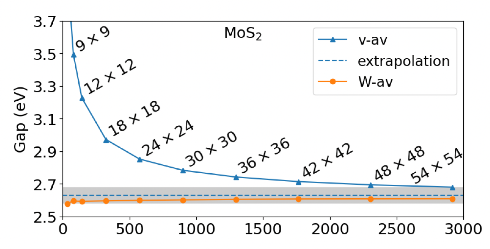
In 2D systems, the improvement granted by the better integration around q=0 of the Coulomb potential via the RIM approach does not work well for the correlation part of self-energy

Convergence of the quasiparticle band gap of MoS2 with respect to the number of sampling points of the BZ. Blue lines: standard integration methods. The extrapolated values are indicated with an horizontal dashed line. Orange lines: RIM-W method. The grey shaded regions show the converge tolerance (±50 meV) centered at the centered at the extrapolated values.

as the dielectric function [math]\displaystyle{ \epsilon_{00} }[/math] goes as q around q=0, matching the 1/q behavior of the Coulomb potential.

To solve this issue, it has been developed a method specific for 2D systems that performs the integration of [math]\displaystyle{ \epsilon_{0 0}(\mathbf{q}) \ v(\mathbf{q}) }[/math] rather than only of [math]\displaystyle{ v(\mathbf{q}) }[/math] when computing the correlation part of self-energy.

Details of this method can be found in the paper Efficient GW calculations in two-dimensional materials through a stochastic integration of the screened potential. You can activate the RIM-W algorithm adding a further flag to your input:

yambo -F gw_ppa.in -p p -r -rw

In your input three further lines should have appeared:

...
rim_cut                           # [R] Coulomb potential
RandQpts=1000000                  # [RIM] Number of random q-points in the BZ
RandGvec= 100              RL     # [RIM] Coulomb interaction RS components
RIM_W
RandGvecW= 15              RL
rimw_type="semiconductor"
...

The variable RandGvecW defines the number of G vectors to integrate W numerically. RandGvecW must be always smaller than the size of the [math]\displaystyle{ \chi }[/math] matrix.

Now repeat the computation again using the RIM-W algorithm.

yambo -F gw_ppa.in -J 80b_10Ry_rimw

How much has the band gap changed ?

Step 2: GW parallel strategies on a cluster

For this part of the tutorial, we will see how to parallelize on a real cluster using gpu. As a test calculation, we compute the full correction to the band structure of single-layer MoS2. In order to get somewhat realistic results, we will use larger values for the convergence parameters with respect the previous calculation. In addition, we also increased the vacuum separation (to 30 au) and the k-point mesh (to 18x18x1) in the DFT calculation, and of course we consider spin-orbit coupling.

Differently to the approach used up to now, we will not work interactively but rather we will submit a job script as is commonly done on clusters.

So now exit the interactive mode and in the login node access

cd $CINECA_SCRATCH/YAMBO_TUTORIALS/MoS2_HPC_tutorial/04_GW_bands

The calculation we want to perform is much heavier than before, and we have to do it not just for the band gap, but the entire band structure which includes 37 kpoints in the irreducible Brillouin zone, two spin-orbit-split valence bands, and two spin-orbit-split conduction bands. Let us check the new input:

vim gw.in

...
%QPkrange                        # [GW] QP generalized Kpoint/Band indices
1|37|25|28|
%
...

This is a massive calculation, so create a job script

vim gpu_job.sh

As you might have guessed from the name of the submission script, we are here using yet another capability of yambo: running on GPUs instead of CPUs. This usually leads to extreme speedups in the calculations. Fortunately, the m100 cluster also has some GPU nodes!

As you can see from the submission script,

vim gpu_job.sh

#!/bin/bash
#SBATCH --nodes=1
#SBATCH --ntasks-per-node=8
#SBATCH --cpus-per-task=1
#SBATCH --gpus-per-node=4

each GPU node contains four GPUs (--gres=gpu:4). In yambo, each GPU corresponds to a single MPI task, therefore we have ntasks-per-node=4. OpenMP threading is allowed - but not too much, otherwise we lose efficiency. and in fact, even though we are filling all CPUs of the node, we are using just `export OMP_NUM_THREADS=8`. Here, we are not using it

In addition, you will see that in order to run on GPUs we are now using a different executable than before, obtained with a GPU-specific compilation of the code.

module purge
module load hpc-sdk/2022--binary spectrum_mpi/10.4.0--binary
export PATH=/m100_work/tra23_Yambo/softwares/YAMBO/5.2-gpu/bin:$PATH

In general, the gpu compilation might be different on your machine, or the executable may be the same with no need to load an additional modules.

In conclusion, we are running over 4 GPU cards, distributed with 8 MPI tasks, and using 4 threads.

After about 6 minutes the calculation should be over and the results collected in folder GW_bnds. The quasiparticle corrections are stored in human-readable form in the file o-GW_bnds.qp, and in netCDF format in the quasiparticle database ndb.QP.