Second-harmonic generation of 2D-hBN: Difference between revisions
Jump to navigation
Jump to search
m (Yambowikiadmin moved page Non-linear response TD-HSEX: hBN to Second-harmonic generation of 2D-hBN) |
No edit summary |
||
| Line 1: | Line 1: | ||
Non linear response | = Step 0: Theoretical framework = | ||
Non-linear response calculations are similar to the linear response case, with the only difference that we excite the system with a sinusoidal external field. A perturbation with a specific frequency allows to expand the polarization in the form <math>\bf{P}(t) = \sum_{n=-\infty}^{+\infty} \bf{p}_n e^{-i\omega_n t} </math> where the coefficient <math>\bf{p}_1,...,\bf{p}_n </math> are related to <math>\chi^{(1)},...,\chi^{(n)} </math>. | |||
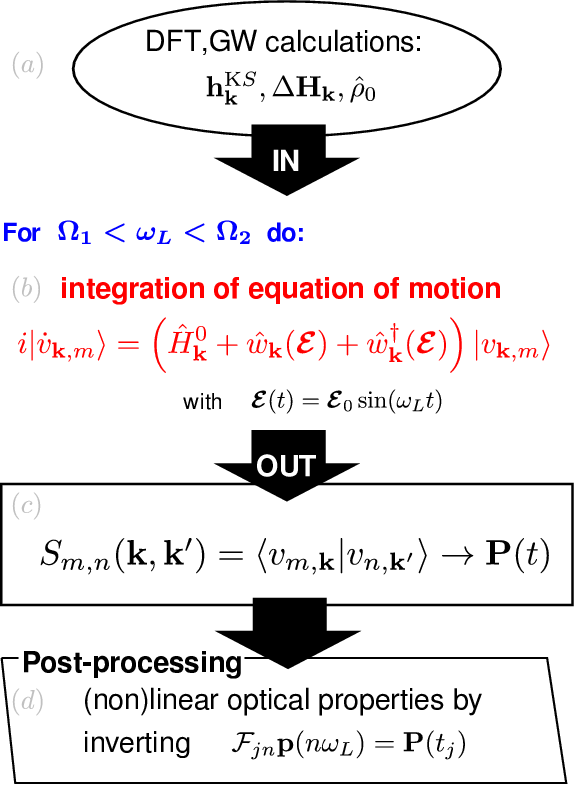
In practice we use the scheme described in Ref. <ref name="Attaccalite2013"></ref> and show below to extract the non-linear coefficients: | |||
[[File:Scheme nl.png|350px|center|Schematic representation of real-time calculations]] | |||
= Step 1: Independent-particle approximation = | |||
= Step 2: Hartree+Screened exchange approximation (BSE level) = | |||
Revision as of 13:37, 19 May 2023
Step 0: Theoretical framework
Non-linear response calculations are similar to the linear response case, with the only difference that we excite the system with a sinusoidal external field. A perturbation with a specific frequency allows to expand the polarization in the form [math]\displaystyle{ \bf{P}(t) = \sum_{n=-\infty}^{+\infty} \bf{p}_n e^{-i\omega_n t} }[/math] where the coefficient [math]\displaystyle{ \bf{p}_1,...,\bf{p}_n }[/math] are related to [math]\displaystyle{ \chi^{(1)},...,\chi^{(n)} }[/math]. In practice we use the scheme described in Ref. [1] and show below to extract the non-linear coefficients:
Step 1: Independent-particle approximation
Step 2: Hartree+Screened exchange approximation (BSE level)
- ↑ Cite error: Invalid
<ref>tag; no text was provided for refs namedAttaccalite2013
