Time-dependent density functional theory (standard kernel): Difference between revisions
| (16 intermediate revisions by one other user not shown) | |||
| Line 1: | Line 1: | ||
In this | In this module you will learn how to calculate optical spectra at the time-dependent density-functional theory level for bulk hBN. | ||
== Background == | == Background == | ||
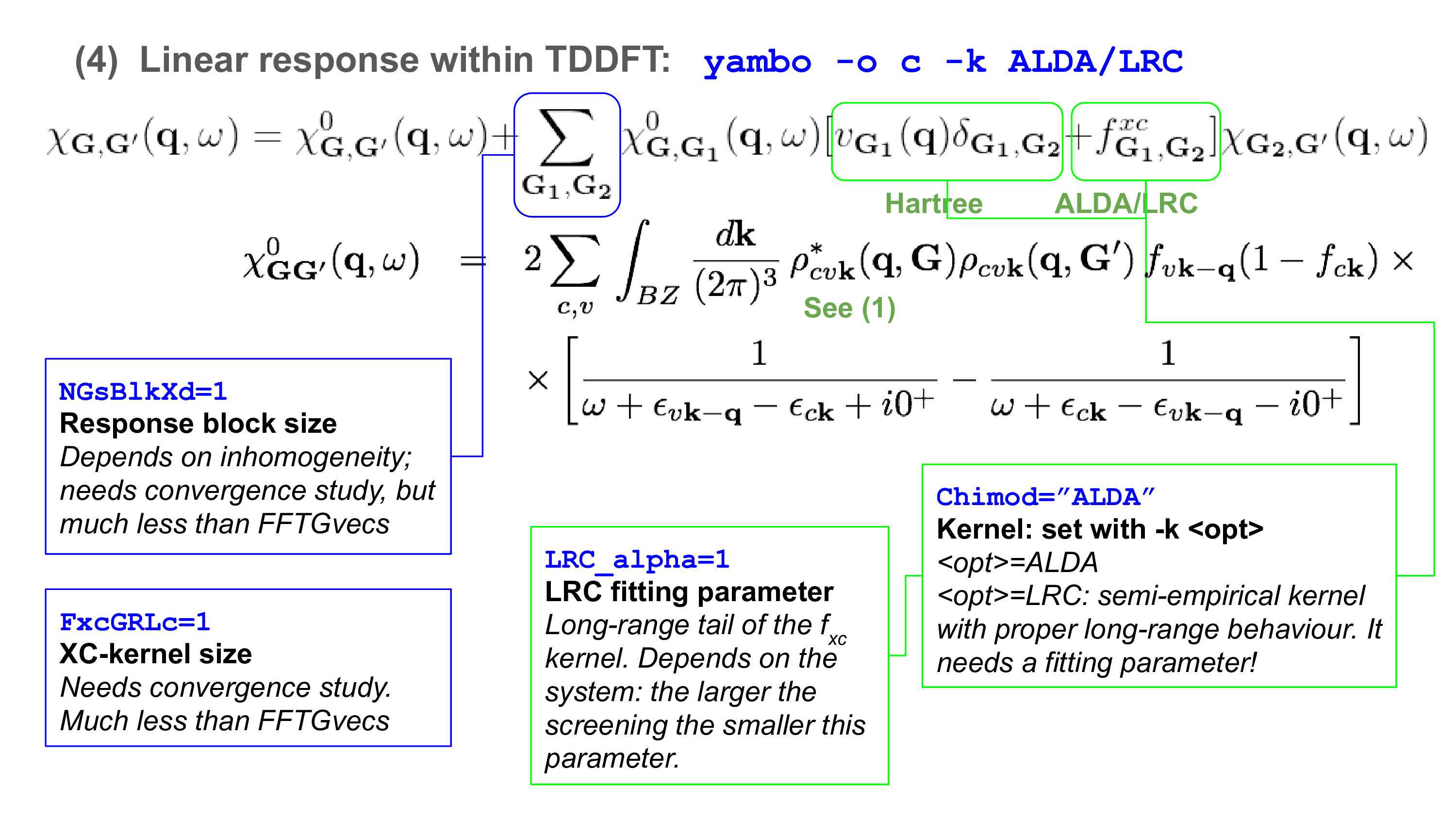
Within the time-dependent DFT formalism the macroscopic dielectric function [[Local_fields|is obtained]] by solving the Dyson equation for the susceptibility ''X''. In reciprocal space this is given by: | |||
[[File:Yambo-CH7.png|none|x50px|Yambo tutorial image]] | [[File:Yambo-CH7.png|none|x50px|Yambo tutorial image]] | ||
The ''f <sup> xc</sup>'' term is called the exchange-correlation (xc) kernel and describes the response of the xc potential at a time ''t'' to changes in the density at all previous times. Approximations | The ''f <sup> xc</sup>'' term is called the exchange-correlation (xc) kernel and describes the response of the xc potential at a time ''t'' to changes in the density at all previous times. Approximations | ||
| Line 15: | Line 9: | ||
Within this family we consider here the adiabatic local density approximation (ALDA) | Within this family we consider here the adiabatic local density approximation (ALDA) | ||
[[File:Eq_ALDA.png|none|x50px]] | [[File:Eq_ALDA.png|none|x50px]] | ||
== Prerequisites == | == Prerequisites == | ||
[[File:Yambo-handbook-v4.1.2-p-5.png|thumb|Cheatsheet on TDDFT|150px]] | |||
* You must first complete the "How to use Yambo" modules | * You must first complete the "How to use Yambo" and the "Optics at the independent particle level" and "local fields" modules | ||
'''You will need''': | '''You will need''': | ||
| Line 35: | Line 20: | ||
== Choosing input parameters == | == Choosing input parameters == | ||
Enter the folder for bulk hBN that contains the | Enter the folder for bulk hBN that contains the SAVE directory, and generate the input file. From <code>yambo -H</code> you should understand that the correct option is <code>yambo -o c -k <opt> </code>. | ||
< | Where <opt> can be 'hartree' as in the tutorial on the [[Local fields|local fields]], or 'alda' or 'lrc' ([[Time-dependent density functional theory (long-range corrected kernel)|see next tutorial]]) respectively for the ALDA and LRC approximations for the xc kernel outlined above. | ||
cd YAMBO_TUTORIALS/hBN/YAMBO | Let's start by generating the input for a calculation with the ALDA kernel: | ||
$ cd YAMBO_TUTORIALS/hBN-3D/YAMBO | |||
yambo | $ yambo ''(Initialization)'' | ||
$ yambo -F yambo.in_ALDA -J 3D_ALDA -o c -k alda | |||
We thus use a new input file ''yambo.in_ALDA'', switch on the <code>FFTGvecs</code> variable, and label all outputs/databases with a ''3D_ALDA'' tag. Make sure to set/modify all of the following variables to: | |||
[[Variables#Chimod|Chimod]]= "ALDA" # [X] IP/Hartree/ALDA/LRC/BSfxc | |||
[[Variables#FxcGRLc|FxcGRLc]]= ''' 3 Ry''' # [Xd] Response block size | |||
[[Variables#NGsBlkXd|NGsBlkXd]]= 3 Ry # [Xd] Response block size | |||
% [[Variables#QpntsRXd|QpntsRXd]] | |||
1 | 1 | # [Xd] Transferred momenta | |||
% | |||
% [[Variables#EnRngeXd|EnRngeXd]] | |||
0.00000 | 10.00000 | eV # [Xd] Energy range | |||
% | |||
% [[Variables#DmRngeXd|DmRngeXd]] | |||
0.200000 | 0.200000 | eV # [Xd] Damping range | |||
% | |||
[[Variables#ETStpsXd|ETStpsXd]]= 1001 # [Xd] Total Energy steps | |||
% [[Variables#LongDrXd|LongDrXd]] | |||
1.000000 | 1.000000 | 0.000000 | # [Xd] [cc] Electric Field | |||
% | |||
In this input file, we have selected: | |||
* the long-wavelength limit q = 0 (optical limit) | |||
* A ''q'' parallel to the BN planes | |||
* The ALDA kernel, and expanded G-vectors in the screening and in the xc kernel up to 3 Ry (about 85 G-vectors) | |||
==Optics runlevel== | ==Optics runlevel== | ||
Save the input file and launch the code, keeping the command line options as before (i.e., just remove the lower case options): | Save the input file and launch the code, keeping the command line options as before (i.e., just remove the lower case options): | ||
$ yambo -F yambo. | $ yambo -F yambo.in_ALDA -J 3D_ALDA | ||
... | ... | ||
< | <01s> [05] Optics | ||
< | <01s> [LA] SERIAL linear algebra | ||
< | <01s> [WF] Performing Wave-Functions I/O from ./SAVE | ||
<01s> [FFT-Rho] Mesh size: 9 9 21 | |||
<01s> [xc] Functional Slater exchange(X)+Perdew & Zunger(C) | |||
<01s> [xc] LIBXC used to calculate xc functional | |||
<01s> [ | |||
<01s> | |||
<01s> [ | |||
... | ... | ||
Note that, with respect to the Hartree kernel (RPA calculations) the libxc is called to calculate the xc kernel within the ALDA, in particular the Perdew-Zunger parametrization for the correlation part of the LDA is used. | |||
Let's compare the absorption with and without the ALDA (+ local fields) included. By inspecting the o-3D-ALDA.eps_q1_inv_rpa_dyson file we find that this information is given in the 2nd and 4th columns, respectively: | |||
$ head -n30 o-3D_ALDA.eps_q1_inv_alda_dyson | |||
# Absorption @ Q(1) [q->0 direction] : 0.7071068 0.7071068 0.0000000 | |||
# E/ev[1] EPS-Im[2] EPS-Re[3] EPSo-Im[4] EPSo-Re[5] | |||
Plot the result: | |||
$ gnuplot | |||
gnuplot> plot "o-3D_ALDA.eps_q1_inv_alda_dyson" u 1:2 w l t 'ALDA',"o-3D_ALDA.eps_q1_inv_alda_dyson" u 1:4 w l t 'IPA' | |||
[[File:3D_ALDA_hBN.png|none|500px|Yambo tutorial image]] | |||
[[File: | |||
What is clear from this plot is that the ALDA kernel does not significantly change the optical spectrum when compared with the independent particle level of approximation (IPA). The same trend can be observed for other semiconductors and insulators. | |||
==Summary== | ==Summary== | ||
From this tutorial you've learned: | From this tutorial you've learned: | ||
* How to compute | * How to compute an optical spectrum within the adiabatic local density approximation | ||
== Links == | == Links == | ||
* Next module: [[ | * Next module: [[Time-dependent density functional theory (long-range corrected kernel) | Long-range corrected kernel]] | ||
* [[Tutorials|Back to tutorials menu]] | * [[Tutorials|Back to tutorials menu]] | ||
Latest revision as of 09:36, 7 November 2019
In this module you will learn how to calculate optical spectra at the time-dependent density-functional theory level for bulk hBN.
Background
Within the time-dependent DFT formalism the macroscopic dielectric function is obtained by solving the Dyson equation for the susceptibility X. In reciprocal space this is given by:
The f xc term is called the exchange-correlation (xc) kernel and describes the response of the xc potential at a time t to changes in the density at all previous times. Approximations for the xc kernel can be derived by taking the functional derivative of common approximations for the xc potential with respect to the density with the additional approximation that only instantaneous changes to the density are considered (adiabatic approximation).
Within this family we consider here the adiabatic local density approximation (ALDA)
Prerequisites
- You must first complete the "How to use Yambo" and the "Optics at the independent particle level" and "local fields" modules
You will need:
- The
SAVEdatabases for bulk hBN - The
yamboexecutable gnuplot, for plotting spectra
Choosing input parameters
Enter the folder for bulk hBN that contains the SAVE directory, and generate the input file. From yambo -H you should understand that the correct option is yambo -o c -k <opt> .
Where <opt> can be 'hartree' as in the tutorial on the local fields, or 'alda' or 'lrc' (see next tutorial) respectively for the ALDA and LRC approximations for the xc kernel outlined above.
Let's start by generating the input for a calculation with the ALDA kernel:
$ cd YAMBO_TUTORIALS/hBN-3D/YAMBO
$ yambo        (Initialization)
$ yambo -F yambo.in_ALDA -J 3D_ALDA -o c -k alda
We thus use a new input file yambo.in_ALDA, switch on the FFTGvecs variable, and label all outputs/databases with a 3D_ALDA tag. Make sure to set/modify all of the following variables to:
Chimod= "ALDA"            # [X] IP/Hartree/ALDA/LRC/BSfxc
FxcGRLc=     3        Ry    # [Xd] Response block size
NGsBlkXd=     3        Ry    # [Xd] Response block size
% QpntsRXd
 1 |  1 |                   # [Xd] Transferred momenta
%
% EnRngeXd
 0.00000 | 10.00000 | eV    # [Xd] Energy range
%
% DmRngeXd
0.200000 | 0.200000 | eV    # [Xd] Damping range
%
ETStpsXd= 1001               # [Xd] Total Energy steps
% LongDrXd
1.000000 | 1.000000 | 0.000000 |        # [Xd] [cc] Electric Field
%
In this input file, we have selected:
- the long-wavelength limit q = 0 (optical limit)
- A q parallel to the BN planes
- The ALDA kernel, and expanded G-vectors in the screening and in the xc kernel up to 3 Ry (about 85 G-vectors)
Optics runlevel
Save the input file and launch the code, keeping the command line options as before (i.e., just remove the lower case options):
$ yambo -F yambo.in_ALDA -J 3D_ALDA
...
<01s> [05] Optics
<01s> [LA] SERIAL linear algebra
<01s> [WF] Performing Wave-Functions I/O from ./SAVE
<01s> [FFT-Rho] Mesh size:  9   9  21
<01s> [xc] Functional Slater exchange(X)+Perdew & Zunger(C)
<01s> [xc] LIBXC used to calculate xc functional
...
Note that, with respect to the Hartree kernel (RPA calculations) the libxc is called to calculate the xc kernel within the ALDA, in particular the Perdew-Zunger parametrization for the correlation part of the LDA is used.
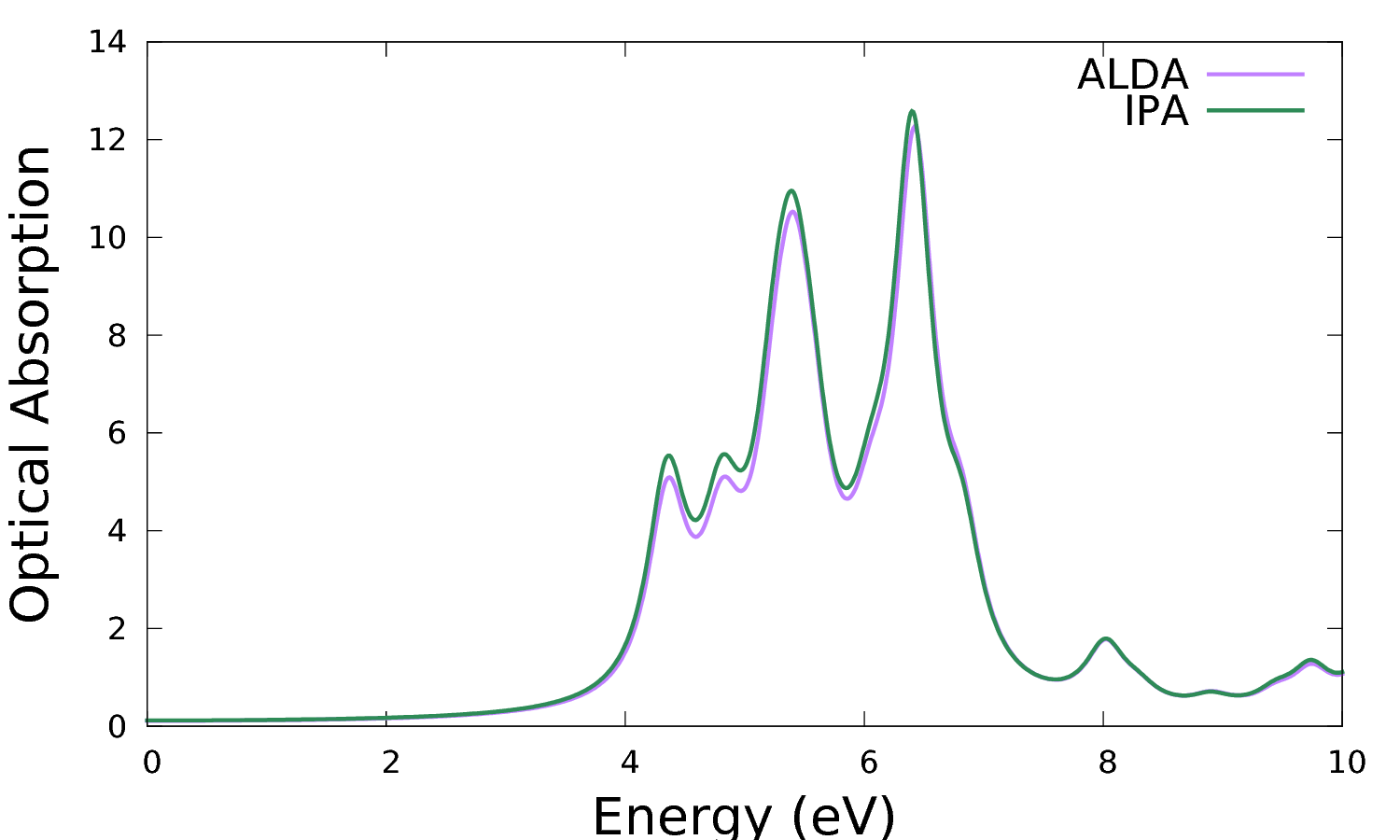
Let's compare the absorption with and without the ALDA (+ local fields) included. By inspecting the o-3D-ALDA.eps_q1_inv_rpa_dyson file we find that this information is given in the 2nd and 4th columns, respectively:
$ head -n30 o-3D_ALDA.eps_q1_inv_alda_dyson
- Absorption @ Q(1) [q->0 direction] : 0.7071068 0.7071068 0.0000000
- E/ev[1] EPS-Im[2] EPS-Re[3] EPSo-Im[4] EPSo-Re[5]
Plot the result:
$ gnuplot gnuplot> plot "o-3D_ALDA.eps_q1_inv_alda_dyson" u 1:2 w l t 'ALDA',"o-3D_ALDA.eps_q1_inv_alda_dyson" u 1:4 w l t 'IPA'
What is clear from this plot is that the ALDA kernel does not significantly change the optical spectrum when compared with the independent particle level of approximation (IPA). The same trend can be observed for other semiconductors and insulators.
Summary
From this tutorial you've learned:
- How to compute an optical spectrum within the adiabatic local density approximation
Links
- Next module: Long-range corrected kernel
- Back to tutorials menu


