Pushing convergence in parallel: Difference between revisions
No edit summary |
(First version) |
||
| Line 1: | Line 1: | ||
== 2D hBN == | |||
In the previous session we focused on the scaling properties of the code. | |||
We now focus more on the physical aspect. | |||
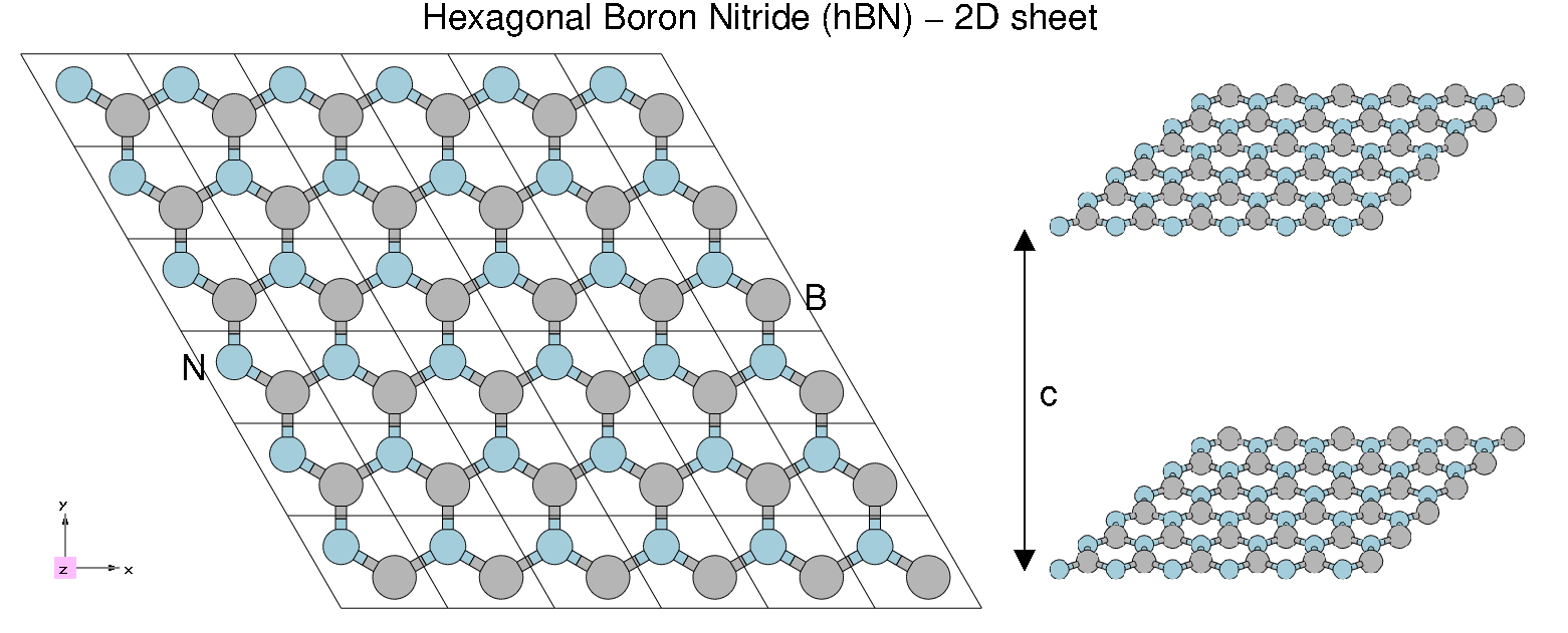
The system we are working on is the 2D-hBN sheet we already used the first day. | |||
[[File:HBN2.png|1000px|center|Atomic structure of 2D hBN]] | [[File:HBN2.png|1000px|center|Atomic structure of 2D hBN]] | ||
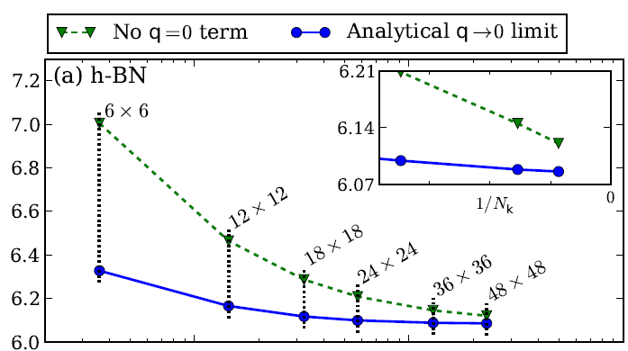
If you wan a published reference of some properties of hBN you can look to the following arxiv, | |||
https://arxiv.org/abs/1511.00129 and references therein were the QP correction are computed. | |||
In that case the convergence with the number of k-points is studied in detail (for hBN and other materials). | |||
The focus is on a proper description of the q->0 limit of the (screened) electron-electron | |||
interaction entering the GW self-energy. Here you can see an image extracted from the arxiv. | |||
As you can see the QP corrections converge slowly with the number of k-points. | |||
[[File:QP convergence hBN from literature.png|600px|center|Yambo tutorial image]] | [[File:QP convergence hBN from literature.png|600px|center|Yambo tutorial image]] | ||
In the present tutorial you will start using a 12x12 grid. | |||
Only in the last part we will re-run pw.x to generate bigger k-grids | |||
Notice that to run convergence you will need to manually change and re-run the input file. | |||
For the k-points case in particular you will need to re-run also pw.x | |||
Tomorrow you will learn how to do that in a more automatic way using the yambopy scripting tools, | |||
however running yambo in serial. | |||
While yambopy offers an easier interface for the use, in the present parallel tutorial you | |||
will be able to push much more the convergence. In a real life calculation you will likely take advantage | |||
of both. | |||
<br> | <br> | ||
Revision as of 22:31, 25 April 2017
2D hBN
In the previous session we focused on the scaling properties of the code. We now focus more on the physical aspect.
The system we are working on is the 2D-hBN sheet we already used the first day.
If you wan a published reference of some properties of hBN you can look to the following arxiv, https://arxiv.org/abs/1511.00129 and references therein were the QP correction are computed. In that case the convergence with the number of k-points is studied in detail (for hBN and other materials). The focus is on a proper description of the q->0 limit of the (screened) electron-electron interaction entering the GW self-energy. Here you can see an image extracted from the arxiv. As you can see the QP corrections converge slowly with the number of k-points.
In the present tutorial you will start using a 12x12 grid. Only in the last part we will re-run pw.x to generate bigger k-grids
Notice that to run convergence you will need to manually change and re-run the input file. For the k-points case in particular you will need to re-run also pw.x Tomorrow you will learn how to do that in a more automatic way using the yambopy scripting tools, however running yambo in serial. While yambopy offers an easier interface for the use, in the present parallel tutorial you will be able to push much more the convergence. In a real life calculation you will likely take advantage of both.
| Prev: Tutorials Home | Now: Tutorials Home --> GW Convergence | Next: Parallel tutorials are over |

